SciPy integration misunderstanding

Today I needed to compute an integral similar to this:

\int_{1000}^\infty \frac{dx}{100, x^3}

I used the following SciPy code to compute the integral:

from scipy.integrate import quad

def f(x):
    return 0.01*x**-3

integral, error = quad(f, 1000, sp.inf, epsrel = 1e-6)
print integral, error

My intention was to compute the integral to 6 significant figures. (epsrel is a shortened form of epsilon relative, i.e. relative error.) To my surprise, the estimated error was larger than the value of the integral. Specifically, the integral was computed as 5.15 × 10⁻⁹ and the error estimate was 9.07 × 10⁻⁹.

What went wrong? The integration routine quad lets you specify either a desired bound on your absolute error (epsabs) or a desired bound on your relative error (epsrel). I assumed that since I specified the relative error, the integration would stop when the relative error requirement was met. But that’s not how it works.

The quad function has default values for both epsabs and epsrel.

def quad(... epsabs=1.49e-8, epsrel=1.49e-8, ...):

I thought that since I did not specify an absolute error bound, the bound was not effective, or equivalently, that the absolute error target was 0. But no! It was as if I’d set the absolute error bound to 1.49 × 10⁻⁸. Because my integral is small (the exact value is 5 × 10⁻⁹) the absolute error requirement is satisfied before the relative error requirement and so the integration stops too soon.

The solution is to specify an absolute error target of zero. This condition cannot be satisfied, and so the relative error target will determine when the integration stops.

integral, error = quad(f, 1000, sp.inf, epsrel = 1e-6, epsabs = 0)

This correctly computes the integral as 5 × 10⁻⁹ and estimates the integration error as 4 ×10⁻¹⁸.

It makes some sense for quad to specify non-zero default values for both absolute and relative error, though I imagine most users expect small relative error rather than small absolute error, so perhaps the latter could be set to 0 by default.

Approximating Earth as a sphere

Isaac Newton suggested in 1687 that the earth is not a perfectly round sphere but rather an ellipsoid, and he was right. But since our planet is roughly a sphere, it’s often useful to approximate it by a sphere. So if you’re going to do that, what radius do you use? More generally, what radius do you use when approximating any ellipsoid by a sphere?

This post will discuss the more general problem of finding the radius when approximating any ellipsoid by a sphere. We will give the answer for Earth in particular, and we’ll show how to carry out the calculations. Most of the calculations are easy, but some involve elliptic integrals and we show how to compute these in Python.

Ellipsoids and spheroids

First of all, what is an ellipsoid? It is a surface whose (x, y, z) coordinates satisfy

\frac{x^2}{a^2} + \frac{y^2}{b^2} + \frac{z^2}{c^2} = 1

Earth is an oblate spheroid, which means a = b > c. Specifically, a = b = 6,378,137 meters, and c = 6,356,752 meters.

If you wanted to approximate an ellipsoid by a sphere, you could use

r = (a + b + c)/3.

Why? Because the knee-jerk reaction whenever you need to reduce a set of numbers to one number is to average them.

Volume of an ellipsoid

We could do a little better, depending on what property of the ellipsoid we’d like to preserve in our approximation. For example, we might want to create a sphere with the same volume as the ellipsoid. In that case we’d use the geometric mean

r = (abc)1/3.

This is because the volume of an ellipsoid is 4πabc/3 and the volume of a sphere is 4πr3/3.

For the particular case of the earth, we’d use

(a2c)1/3 = 6371000.7

Surface area of an ellipsoid

For some applications we might want a sphere with the same surface area as the ellipsoid rather than the same volume.

The surface area of an ellipsoid is considerably more complicated than the volume. For the special case of an oblate spheroid, like earth, the area is given by

2\pi a^2 \left( 1 + \frac{1 - e^2}{e} \tanh^{-1}e \right)

where

e^2 = 1 - \frac{c^2}{a^2}

The surface area of a sphere is 4 πr2 and so the following code computes r.

    from math import sqrt, atanh
    e = sqrt(1 - (c/a)**2)
    r = a*sqrt(1 + (1-e**2)*atanh(e)/e) / sqrt(2)

This gives r = 6371007.1 for the earth, about 6.4 meters more than the number we got matching volume rather than area.

For a general ellipsoid, the surface area is given by

2\pi c^2 + \frac{2\pi a b}{\sin \varphi} \left( E(\varphi, k) \sin^2\varphi + F(\varphi, k) \cos^2 \varphi\right)

where

cos \varphi = \frac{c}{a}

and

k^2 = \frac{a^2(b^2 - c^2)}{b^2(a^2 - c^2)}

Here F is the “incomplete elliptic integral of the first kind” and E is the “incomplete elliptic integral of the second kind.” The names are historical artifacts, but the “elliptic” part of name comes from the fact that these functions were discovered in the context of arc lengths with ellipses, so it shouldn’t be too surprising to see them here.

Computing ellipsoid surface area in Python

In SciPy, F(φ, k) is given by ellipkinc and E(φ, k) is given by ellipeinc. Both function names start with ellip because they are elliptic functions, and end in inc because they are “incomplete.” In the middle, ellipeinc has an “e” because it computes the mathematical function E(φ, k).

But why does ellipkinc have a “k” in the middle? The “complete” elliptic integral of the first kind is K(k) = F(π/2, k). The “k” in the function name is a reminder that we’re computing the incomplete version of the K function.

Here’s the code for computing the surface area of a general ellipsoid:

    from math import sin, cos, acos, sqrt, pi
    from scipy.special import ellipkinc, ellipeinc

    def area(a, b, c):
        phi = acos(c/a)
        k = a*sqrt(b**2 - c**2)/(b*sqrt(a**2 - c**2))
        E = ellipeinc(phi, k)
        F = ellipkinc(phi, k)
        elliptic = E*sin(phi)**2 + F*cos(phi)**2
        return 2.0*pi*c**2 + 2*pi*a*b*elliptic/sin(phi)

The differences between the various approximation radii are small for Earth. See my next post on elliptical galaxies where the differences are much larger.

More geodesy posts

How to compute jinc(x)

The function jinc(x) that I wrote about yesterday is almost trivial to implement, but not quite. I’ll explain why it’s not quite as easy as it looks and how one might implement it in C and Python.

The function jinc(x) is defined as J1(x) / x, so if you have code to compute J1 then it ought to be a no-brainer. For example, why not use the following C code?

    #include <math.h>
    double jinc(double x) {
        return j1(x) / x;
    }

The problem is that if you pass in 0, the code will divide by 0 and return a NaN. The function jinc(x) is defined to be 1/2 at x = 0 because that’s the limit of J1(x)(x) / x as x goes to 0. So we try again:

    #include <math.h>
    double jinc(double x) {
        return (x == 0.0) ? 0.5 : j1(x) / x;
    }

Does that work? Technically, it could still fail — we’ll come back to that at the end — but we’ll assume for now that it’s OK.

We could write the analogous Python code, and it would be adequate as long as we’re only calling the function with scalars and not NumPy arrays.

    from scipy.special import j1
    def jinc(x):
        if x == 0.0:
            return 0.5
        return j1(x) / x

Now suppose you want to plot this function. You create an array of points, say

    x = np.linspace(-1, 1, 25)

and plot jinc(x). You’ll get a warning: “ValueError: The truth value of an array with one element is ambiguous. Use a.any() or a.all().” Incidentally, if we called linspace with an even integer in the last argument, our array of points would avoid zero and the naive implementation of jinc would work.

When Python tries to apply jinc to an array, it doesn’t know how to interpret the test x == 0. The warning suggests “Do you mean if any component of x is 0? Or if all components of x are 0?” Neither option is what we want. We want to apply jinc as written to each element of x. We could do this by calling the vectorize function.

    jinc = np.vectorize(jinc)

This replaces our original jinc function with one that handles NumPy arrays correctly.

There is an extremely unlikely scenario in which the code above could fail. The value of J1(x) is approximately x/2 for small values of x. If the floating point value x is so small that 0.5*x returns 0, our function will return 0, even though it should return 0.5. The C code above works for values of x as small as DBL_MIN and even values much smaller. (DBL_MIN is not the smallest value of a double, only the smallest normalized double.) But if you set

    x = DBL_MIN / pow(2.0, 52);

then jinc(x) will return 0. If you want to be absolutely safe, you could change the implementation to

    #include <math.h>
    double jinc(double x) {
        return (fabs(x) < 1e-8) ? 0.5 : j1(x) / x;
    }

Why test for whether the absolute value is less than 10−8 rather than a much smaller number? For small x, the error in approximating jinc(x) with 1/2 is on the order of x2/16. So for x as large as 10−8, the approximation error is below the resolution of a double. As a bonus, the function jinc(x) will be more efficient for |x| < 10−8 since it avoids a call to j1.

Related posts

Benford’s law and SciPy

Imagine you picked up a dictionary and found that the pages with A’s were dirty and the Z’s were clean. In between there was a gradual transition with the pages becoming cleaner as you progressed through the alphabet. You might conclude that people have been looking up a lot of words that begin with letters near the beginning of the alphabet and not many near the end.

That’s what Simon Newcomb did in 1881, only he was looking at tables of logarithms. He concluded that people were most interested in looking up the logarithms of numbers that began with 1 and progressively less interested in logarithms of numbers beginning with larger digits. This sounds absolutely bizarre, but he was right. The pattern he described has been repeatedly observed and is called Benford’s law. (Benford re-discovered the same principle in 1938, and per Stigler’s law, Newcomb’s observation was named after Benford.)

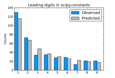
Benford’s law predicts that for data sets such as collections of physical constants, about 30% of the numbers will begin with 1 down to about 5% starting with 8 or 9. To be precise, it says the leading digit will be d with probability log10(1 + 1/d). For a good explanation of Benford’s law, see TAOCP volume 2.

A couple days ago I blogged about using SciPy’s collection of physical constants to look for values that were approximately factorials. Let’s look at that set of constants again and see whether the most significant digits of these constants follows Benford’s law.

Here’s a bar chart comparing the actual number of constants starting with each digit to the results we would expect from Benford’s law.

Here’s the code that was used to create the data for the chart.

from math import log10, floor
from scipy.constants import codata

def most_significant_digit(x):
    e = floor(log10(x))
    return int(x*10**-e)

# count how many constants have each leading digit
count = [0]*10
d = codata.physical_constants
for c in d:
    (value, unit, uncertainty) = d[ c ]
    x = abs(value)
    count[ most_significant_digit(x) ] += 1
total = sum(count)

# expected number of each leading digit per Benford's law
benford = [total*log10(1 + 1./i) for i in range(1, 10)]

The chart itself was produced using matplotlib, starting with this sample code.

The actual counts we see in scipy.constants line up fairly well with the predictions from Benford’s law. The results are much closer to Benford’s prediction than to the uniform distribution that you might have expected before hearing of Benford’s law.

Update: See the next post for an explanation of why factorials also follow Benford’s law.

Related posts

Physical constants and factorials

The previous post mentioned that Avogadro’s constant is approximately 24!. Are there other physical constants that are nearly factorials?

I searched SciPy’s collection of physical constants looking for values that are either nearly factorials or nearly reciprocals of factorials.

The best example is the “classical electron radius” re which is 2.818 × 10⁻¹⁵ m and 1/17! = 2.811 × 10⁻¹⁵.

Also, the “Hartree-Hertz relationship” Eh/h equals 6.58 × 10¹⁵ and 18! = 6.4 × 10¹⁵. (Eh is the Hartree energy and h is Plank’s constant.)

Here’s the Python code I used to discover these relationships.

from scipy.special import gammaln
from math import log, factorial
from scipy.optimize import brenth
from scipy.constants import codata

def inverse_factorial(x):
    # Find r such that gammaln(r) = log(x)
    # So gamma(r) = x and (r-1)! = x
    r = brenth(lambda t: gammaln(t) - log(x), 1.0, 100.0)
    return r-1

d = codata.physical_constants
for c in d:

    (value, unit, uncertainty) = d[ c ]
    x = value
    if x < 0: x = abs(x)
    if x < 1.0: x = 1.0/x
    r = inverse_factorial(x)
    n = round(r)
    # Use n > 6 to weed out uninteresting values.
    if abs(r - n) < 0.01 and n > 6:
        fact = factorial(n)
    if value < 1.0:
        fact = 1.0/fact
    print c, n, value, fact

Python for high performance computing

William Scullin’s talk from PyCon 2011: Python for high performance computing.

At least in our shop [Argonne National Laboratory] we have three accepted languages for scientific computing. In this order they are C/C++, Fortran in all its dialects, and Python. You’ll notice the absolute and total lack of Ruby, Perl, Java.

If you’re interested in Python and HPC, check out SciPyTip.

Ruby, Python, and Science

David Jacobs has written a long blog post Ruby is beautiful (but I’m moving to Python). [Update: link no longer available.] Here’s my summary.

Ruby is much better than Java, but the Ruby community is too focused on web development and the language has no scientific library. Python has a lot of the same advantages as Ruby, is used for more than web programming, and has SciPy.

Update: There is now a fledgling SciRuby project.

Further reading

Bug in SciPy’s erf function

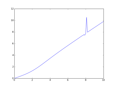
Last night I produced the plot below and was very surprised at the jagged spike. I knew the curve should be smooth and strictly increasing.

My first thought was that there must be a numerical accuracy problem in my code, but it turns out there’s a bug in SciPy version 0.8.0b1. I started to report it, but I saw there were similar bug reports and one such report was marked as closed, so presumably the fix will appear in the next release.

The problem is that SciPy’s erf function is inaccurate for arguments with imaginary part near 5.8. For example, Mathematica computes erf(1.0 + 5.7i) as -4.5717×10¹² + 1.04767×10¹² i. SciPy computes the same value as -4.4370×10¹² + 1.3652×10¹² i. The imaginary component is off by about 30%.

Here is the code that produced the plot.

from scipy.special import erf
from numpy import linspace, exp
import matplotlib.pyplot as plt

def g(y):
    z = (1 + 1j*y) /  sqrt(2)
    temp = exp(z*z)*(1 - erf(z))
    u, v = temp.real, temp.imag
    return -v / u

x = linspace(0, 10, 101)
plt.plot(x, g(x))

Moving from Mathematica to Python

Everything I do regularly in Mathematica can be done in Python. Even though Mathematica has a mind-boggling amount of functionality, I only use a tiny proportion of it. I skimmed through some of my Mathematica files to see what functions I use and then looked for Python counterparts. I found I use less of Mathematica than I imagined.

The core mathematical functions I need are in SciPy. The plotting features are in matplotlib. The SymPy library appears to have the symbolic functionality I need, though I’m as not sure about this one.

As I’ve blogged about before, I’d like to consolidate my tools. I started using Emacs again because I was frustrated with using a different editor for every kind of file. One of the things I find promising about Python is that I may be able to do more in Python and reduce the number of programming languages I use regularly.

Update (2017):

I wrote this post years ago when I was just starting to move to the Python stack. Since that time I have used Python as my default programming environment, though I still use Mathematica as well. The number and quality of Python libraries for applied mathematics has increased greatly over that time.

Python has numerous advantages over Mathematica. It is open source, and so it is more transparent. When something goes wrong, you can dig in and debug it. It is of course free, so you don’t have to buy software licenses, saving not only money but administrative hassle. And perhaps more importantly, other people that you want to share code with don’t have to buy licenses; you might find a Mathematica license a good investment for your company, but you can’t expect everyone you work with to necessarily come to the same conclusion.

The disadvantage to Python relative to Mathematica is that it is less consistent and less integrated. The Python stack for applied math—SciPy, NumPy, Pandas, Matplotlib, etc.—is better integrated than it used to be, but it still remains a collection of separate libraries.