Random inequalities

My previous post introduced random inequalities and their application to Bayesian clinical trials. This post will discuss how to evaluate random inequalities analytically. The next post in the series will discuss numerical evaluation when analytical evaluation is not possible.

For independent random variables X and Y, how would you compute P(X>Y), the probability that a sample from X will be larger than a sample from Y? Let f_X be the probability density function (PDF) of X and let F_X be the cumulative distribution function (CDF) of X. Define f_Y and F_Y similarly. Then the probability P(X > Y) is the integral of f_X(x) f_Y(y) over the part of the x–y plane below the diagonal line x = y.

$\begin{eqnarray*} P(X \geq Y) &=& \int \!\int _{[x > y]} f_X(x) f_Y(y) \, dy \, dx \\ &=& \int_{-\infty}^\infty \! \int_{-\infty}^x f_X(x) f_Y(y) \, dy \, dx \\ &=& \int_{-\infty}^\infty f_X(x) F_Y(x) \, dx \end{eqnarray*}$

This result makes intuitive sense: f_X(x) is the density for x and F_Y(x) is the probability that Y is less than x. Sometimes this integral can be evaluated analytically, though in general it must be evaluated numerically. The technical report Numerical computation of stochastic inequality probabilities explains how P(X > Y) can be computed in closed form for several common distribution families as well as how to evaluate inequalities involving other distributions numerically.

Exponential: If X and Y are exponential random variables with mean μ_X and μ_Y respectively, then P(X > Y) = μ_X/(μ_X + μ_Y).

Normal: If X and Y are normal random variables with mean and standard deviation (μ_X, σ_X) and (μ_Y, σ_Y) respectively, then P(X > Y) = Φ((μ_X – μ_Y)/√(σ_X² + σ_Y²)) where Φ is the CDF of a standard normal distribution.

Gamma: If X and Y are gamma random variables with shape and scale (α_X, β_X) and (α_Y, β_Y) respectively, then P(X > Y) = I_x(β_X/(β_X + β_Y)) where I_x is the incomplete beta function with parameters α_Y and α_X, i.e. the CDF of a beta distribution with parameters α_Y and α_X.

The inequality P(X > Y) where X and Y are beta random variables comes up very often in applications. This inequality cannot be computed in closed form in general, though there are closed-form solutions for special values of the beta parameters. If X ~ beta(a, b) and Y ~ beta(c, d), the probability P(X > Y) can be evaluated in closed form if

one of the parameters a, b, c, or d is an integer,
a + b + c + d = 1, or
a + b = c + d = 1.

These last two cases can be combined with a recurrence relation to compute other probabilities. See Exact calculation of beta inequalities for more details.

Sometimes you need to calculate P(X > max(Y, Z)) for three independent random variables. This comes up, for example, when computing adaptive randomization probabilities for a three-arm clinical trial. For a time-to-event trial as implemented here, the random variables have a gamma distribution. See Numerical evaluation of gamma inequalities for analytical as well as numerical results for computing P(X > max(Y, Z)) in that case.

The next post in this series will discuss how to evaluate random inequalities numerically when closed-form integration is not possible.

Update: See Part IV of this series for results with the Cauchy distribution.

Many Bayesian clinical trial methods have at their core a random inequality. Some examples from M. D. Anderson: adaptive randomization, binary safety monitoring, time-to-event safety monitoring. These method depends critically on evaluating P(X > Y) where X and Y are independent random variables. Roughly speaking, P(X > Y) is the probability that the treatment represented by X is better than the treatment represented by Y. In a trial with binary outcomes, X and Y may be the posterior probabilities of response on each treatment. In a trial with time-to-event outcomes, X and Y may be posterior probabilities of median survival time on two treatments.

People often have a little difficulty understanding what P(X > Y) means. What does it mean? If we take a sample from X and a random sample from Y, P(X >Y) is the probability that the former is larger than the latter. Most confusion around random inequalities comes from thinking of random variables as constants, not random quantities. Here are a couple examples.

First, suppose X and Y have normal distributions with standard deviation 1. If X has mean 4 and Y has mean 3, what is P(X > Y)? Some would say 1, because X is bigger than Y. But that’s not true. X has a larger mean than Y, but fairly often a sample from Y will be larger than a sample from X. P(X > Y) = 0.76 in this case.

Next, suppose X and Y are identically distributed. Now what is P(X > Y)? I’ve heard people say zero because the two random variables are equal. But they’re not equal. Their distribution functions are equal but the two random variables are independent. P(X > Y) = 1/2 by symmetry.

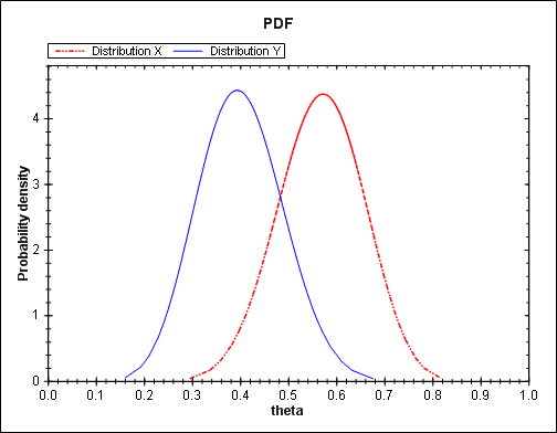
I believe there’s a psychological tendency to underestimate large inequality probabilities. (I’ve had several discussions with people who would not believe a reported inequality probability until they computed it themselves. These discussions are important when the decision whether to continue a clinical trial hinges on the result.) For example, suppose X and Y represent the probability of success in a trial in which there were 17 successes out of 30 on X and 12 successes out of 30 on Y. Using a beta distribution model, the density functions of X and Y are given below.

beta inequality graph

The density function for X is essentially the same as Y but shifted to the right. Clearly P(X > Y) is greater than 1/2. But how much greater than a half? You might think not too much since there’s a lot of mass in the overlap of the two densities. But P(X > Y) is a little more than 0.9.

The image above and the numerical results mentioned in this post were produced by the Inequality Calculator software.

Part II will discuss analytically evaluating random inequalities. Part III will discuss numerically evaluating random inequalities.

Random inequalities II: analytical results

Random inequalities I: introduction