The conjugate of a complex number

is the complex number

Taking the conjugate flips over a complex number, taking its reflection in the real axis.

Multiplication stretches and rotates complex numbers, and addition translates complex numbers. You can’t flip the complex plane over by any series of dilatations, rotations, and translations.

The situation is different for quaternions. The conjugate of a quaternion

is

You can flip four dimensional space over by a series of dilations, rotations, and translations. Namely

To prove this equation, let’s first see what happens when you multiply q on both sides by i:

That is, the effect of multiplying on both sides by i is to flip the sign of the real component and the i component.

Multiplying on both sizes by j or k works analogously: it flips the sign of the real component and its component, and leaves the other two alone.

It follows that

and so the result follows from dividing by −2.

Update: There’s an analogous theorem for octonions.

More on quaternions

• Quaternion square roots
• How close are quaternions to commuting?
• Quaternions and Paradise Lost

Pick a quaternion

p = p₀ + p₁i + p₂j + p₃k

and consider the function that acts on quaternions by multiplying them on the left by p.

If we think of q as a vector in R⁴ then this is a linear function of q, and so it can be represented by multiplication by a 4 × 4 matrix M_p.

It turns out

How might you remember or derive this matrix? Consider the matrix on the left below. It’s easier to see the pattern here than in M_p.

You can derive M_p from this matrix.

Let’s look at the second row, for example. The second row of M_p, when multiplied by q as a column vector, produces the i component of the product.

How do you get an i term in the product? By multiplying the i component of p by the real component of q, or by multiplying the real component of p times the i component of p, or by multiplying the i/ j component of p by the j component of q, or by multiplying the i/k component of p by the k component of q.

The other rows follow the same pattern. To get the x component of the product, you add up the products of the x/y term of p and the y term of q. Here x and y range over

{1, i, j, k}.

To get M_p from the matrix on the right, replace 1 with the real component of p, replace i with the i component of p, etc.

As a final note, notice that the off-diagonal elements of M_p are anti-symmetric:

m_ij = –m_ji

unless i = j.

A couple days ago I wrote about Gauss’ trick to multiply two complex numbers using only 3 real multiplications. This post will do something similar with quaternions.

Just as the most direct approach to computing complex products requires 4 real multiplications, the most direct approach to quaternion products requires 16 real multiplications. (See the function mult here.)

We can represent a quaternion as a pair of complex numbers by observing

a + bi + cj + dk = (a + bi) + (c + di)j

Gauss’ trick can multiply two complex numbers using only three real multiplications. It would seem that we could use something analogous to multiply two quaternions using only 3 complex multiplications, then apply Gauss’ trick to do each of these complex multiplications with 3 real multiplications. The net result would be computing a quaternion product in only 9 real multiplications.

Except that doesn’t work. A direct application of Gauss’ trick doesn’t work because i and j don’t commute. Perhaps there’s some variation on Gauss’ trick that would work, but I haven’t found one.

So let’s back up and take a different approach.

You can represent the quaternions as 2 × 2 complex matrices via

So we could multiply two quaternions by multiplying two 2 × 2 complex matrices. That would require 8 complex multiplications [1], which could be carried out using 3 real multiplications each. This would let us “reduce” the number of multiplications from 16 to 24.

But by symmetry we could eliminate half the multiplications. This puts us at 12 real multiplications, which is less than the 16 required by the most direct approach.

To see this, let α = a − di and β = c + bi. Then our matrix representation has the form

Then our quaternion product becomes the matrix product

We only need to compute the complex products in top row; we can recover the quaternion representation of the product from there. The products in the second row are negatives or conjugates of products in the first row.

Maybe there’s a Gauss-like trick to compute the top row of the matrix using only three complex products, but it can at least be done using four complex products.

Related posts

• How to compute the square root of a complex number
• Octonion and sedenion multiplication

[1] You could use Strassen’s approach to multiply two 2 × 2 matrices in 7 multiplications. That would cut the number of real multiplications down to 21, but exploiting symmetry cuts the number of multiplications further.

You can use quaternions to describe rotations and quaternion products to carry out these rotations. These products have the form

qpq*

where q represents a rotation, q* is its conjugate, and p is the the vector being rotated. (That’s leaving out some details that we’ll get to shortly.)

The primary advantage of using quaternions to represent rotations is that it avoids gimbal lock, a kind of coordinate singularity.

Saving multiplications

If you multiply quaternions directly from the definitions, the product takes 16 real multiplications. (See the function mult in the Python code below.) So a naive implication of the product above, with two quaternion multiplications, would require 32 real multiplications.

You can do something analogous to Gauss’s trick for complex multiplication to do each quaternion product with fewer multiplications [1, 2], but there’s an even better way. It’s possible to compute the rotation in 15 multiplications [3].

Details

Before we can say what the faster algorithm is, we have to fill in some details we left out at the top of the post. We’re rotating a vector in 3 dimensions using quaternions that have 4 dimensions. We do that by embedding our vector in the quaternions, carrying out the product above, and then pulling the rotated vector out.

Specifically, let

v = (v₁, v₂, v₃)

be the vector we want to rotate. We turn v into a quaternion by defining

p = (o, v₁, v₂, v₃).

We encode our rotation in the unit quaternion

q = (q₀, q₁, q₂, q₃)

where q₀ = cos(θ/2) and (q₁, q₂, q₃) is the axis we want to rotate around and θ is the amount we rotate.

The rotated vector is the vector part of

qpq*

i.e. the vector formed by chopping off the first component of the quaternion product.

Algorithm

Let

t = 2 (q₁, q₂, q₃) × (v₁, v₂, v₃) = (t₁, t₂, t₃)

where × is cross product. Then the rotated vector is

v‘ = (v₁, v₂, v₃) + q₀(t₁, t₂, t₃) + (q₁, q₂, q₃) × (t₁, t₂, t₃).

The algorithm involves two cross products, with 6 real multiplications each, and one scalar-vector product requiring 3 real multiplications, for a total of 15 multiplications. (I’m not counting the multiplication by 2 as a multiplications because it could be done by an addition or by a bit-shift.)

Code

Here’s some Python code to carry out the naive product and the faster algorithm.

    import numpy as np

    def mult(x, y):
        return np.array([
            x[0]*y[0] - x[1]*y[1] - x[2]*y[2] - x[3]*y[3],
            x[0]*y[1] + x[1]*y[0] + x[2]*y[3] - x[3]*y[2],
            x[0]*y[2] - x[1]*y[3] + x[2]*y[0] + x[3]*y[1],
            x[0]*y[3] + x[1]*y[2] - x[2]*y[1] + x[3]*y[0]
        ])

    def cross(x, y):
        return np.array( (x[1]*y[2] - x[2]*y[1], x[2]*y[0] - x[0]*y[2], x[0]*y[1] - x[1]*y[0]) )

    def slow_rot(q, v):
        qbar = -q
        qbar[0] = q[0]
        return mult(mult(q, v), qbar)[1:]

    def fast_rot(q, v):
        t = 2*cross(q[1:], v[1:])
        return v[1:] + q[0]*t + cross(q[1:], t)

And here’s some test code.

    def random_quaternion():
        x = np.random.normal(size=4)
        return x 

    for n in range(10):
        v = random_quaternion()
        v[0] = 0
        q = random_quaternion()
        q /= np.linalg.norm(q)
        vprime_slow = slow_rot(q, v)
        vprime_fast = fast_rot(q, v)
        print(vprime_fast - vprime_slow)

This prints 10 vectors that are essentially zero, indicating that vprime_slow and vprime_fast produced the same result.

It’s possible to compute the rotation in less time than two general quaternion products because we had three things we could exploit.

1. The quaternions q and q* are very similar.
2. The first component of p is zero.
3. We don’t need the first component of qpq*, only the last three components.

Related posts

• Advantages to redundant coordinates
• Quaternion square roots
• Average of xy – yx for quaternions

[1] I know you can multiply quaternions using 12 real multiplications, and I suspect you can get it down to 9. See this post.

[2] Note that I said “fewer multiplications” rather than “faster.” Gauss’ method eliminates a multiplication at the expense of 3 additions. Whether the re-arranged calculation is faster depends on the ratio of time it takes for a multiply and an add, which depends on hardware.

However, the rotation algorithm given here reduces multiplications and additions, and so it should be faster on most hardware.

[3] I found this algorithm here. The author cites two links, both of which are dead. I imagine the algorithm is well known in computer graphics.

If y is a quaternion, how many solutions does x² = y have? That is, does every quaternion have a square root, and if so, how many square roots does it have?

A quaternion can have more than two roots. There is a example right in the definition of quaternions:

i² = j² = k² = -1

and so -1 has at least three square roots. It follows that every negative real number has at least three square roots.

Negative reals

In fact, every square root of -1 corresponds to a square root of any other negative number. To see this, let p be a positive real number and let r = √p > 0. If x is a square root of -1, then rx is a square root of –p. Conversely, if x is a square root of –p, then x/r is a square root of -1.

So all negative real numbers have the same number of square roots in the quaternions, and that number is at least 3. In fact, it turns out that all negative real numbers have infinitely many quaternion roots. A calculation shows that

(a + bi + cj + dk)² = -1

if and only if b² + c² + d² = 1. So there are as many square roots of -1 as there are points on a sphere.

Not negative reals

If a quaternion is not a negative real number, then the story is much more familiar: the equation x² = y has one solution if y = 0 and two solutions otherwise.

To summarize, x² = y has

• one solution if y = 0,
• infinitely many solutions if y is negative and real, and
• two solutions otherwise.

It’s easy to show that 0 has only one root: |x²| = |x|², and so if x² = 0, then |x| = 0 and so x = 0. Here the norm of a quaternion is defined by

|a + bi + cj + dk| = √(a² + b² + c² + d²).

If p > 0, the solutions to x² = –p are bi + cj + dk where b² + c² + d² = p.

What’s left is to show that if y is not zero and not a negative real, then x² = y has two solutions.

Polar form and calculating roots

Quaternions have a polar form analogous to the polar form for complex numbers. That is, we can write a quaternion y in the form

y = r(cos θ + u sin θ)

where r is real and positive, θ is real, and u is a unit quaternion with zero real part. We can find r, θ, and u as follows. Write y as

a + bi + cj + dk = a + q

so that a is the real part and q is the pure quaternion part. Then we can find r, θ, and u by

r = |y|
cos θ = a/|y|
u = q / |q|

Then the two roots are

x = ±√r (cos θ/2 + u sin θ/2).

Python code

First we’ll implement the algorithm above, then show that it produces the same results as the Python package quaternionic.

First, our code to compute x satisfying x² = y.

    import numpy as np

    np.random.seed(20210106)

    def norm(q):
        return sum(t*t for t in q)**0.5

    y = np.random.random(size=4)
    r = norm(y)
    theta = np.arccos(y[0]/r)

    u = y + 0 # make a copy
    u[0] = 0
    u /= norm(u)

    x = np.sin(theta/2)*u
    x[0] = np.cos(theta/2)
    x *= r**0.5

And now we check our results using quaternionic.

    import quaternionic

    qx = quaternionic.array(x)
    qy = quaternionic.array(y)

    print(f"y   = {y}")
    print(f"x*x = {qx*qx}")       # should equal y
    print(f"x   = {x}")           # our root
    print(f"x   = {np.sqrt(qy)}") # root via package

This produces

    y   = [0.61615367 0.07612092 0.09606777 0.11150865]
    x*x = [0.61615367 0.07612092 0.09606777 0.11150865]
    x   = [0.79189641 0.04806243 0.06065678 0.07040609]
    x   = [0.79189641 0.04806243 0.06065678 0.07040609]

More quaternion posts

• Finnegans Wake and quaternions
• How far is xy from yx on average for quaternions?
• Probability of commuting

For an exploration of the roots of general polynomial equations over polynomials, see Equations in Quaternions by Ivan Niven. The American Mathematical Monthly, Dec., 1941, Vol. 48, pp. 654-661.

To contemporary ears “quaternion” refers to a number system discovered in the 19h century, but there were a couple precedents. Both refer to something related to a group of four things, but there is no relation to mathematical quaternions other than that they have four dimensions.

I’ve written before about Milton’s use of the word in Paradise Lost. Milton is alluding to the four elements of antiquity: air, earth, fire, and water.

I recently found out the word quaternion appears in the Latin Vulgate as well. Acts 12:4 records that Herod had Peter guarded by four squads of four soldiers each, “quattuor quaternionibus militum.”

Update: Thanks to Phil for pointing out in the comments that quaternion appears in the King James as well, “four quaternions of soldiers.”

More quaternion posts

• How far is xy from yx on average for quaternions?
• Dot product, cross product, and quaternion product
• Beyond quaternions: octonions and sedenions

The blog post that kicked off the recent series of posts looked at how far apart xy and yx are for quaternions. There I used the Euclidean distance, i.e. || xy − yx ||. This time I’ll look at the angle between xy and yx, and I’ll make some analogous graphs for octonions.

For vectors x and y in three dimensions, the dot product satisfies

where θ is the angle between the two vectors. In higher dimensions, we can turn this theorem around and use it as the definition of the angle between two vectors based on their dot product.

(The plots below are jagged because they’re based on random sampling.)

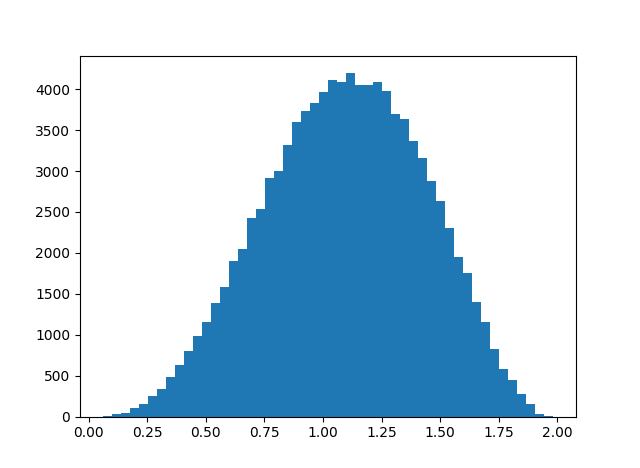
Here’s the Euclidean distance between xy and yx for quaternions from the earlier post:

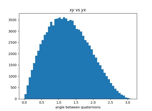
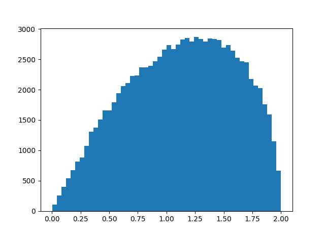
And here’s the corresponding angular distance:

The range has changed from [0, 2] to [o, π], and the distribution now shifts left instead of right.

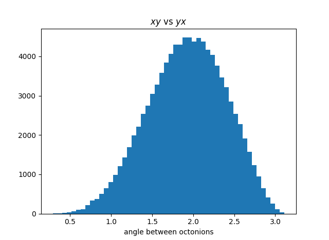
Here’s a similar graph, looking at the angular distance between xy and yx for octonions, something I haven’t plotted before in Euclidean distance.

This graph is more symmetric, which we might expect: since octonions have less algebraic structure than quaternions, we might expect the relationship between xy and yz to behave more erratically, and for the plot to look more like a normal distribution.

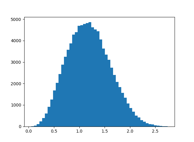
Finally, let’s revisit the distance between (xy)z and x(yz) for octonions. Here is the distribution of the Euclidean distance from a previous post:

And here is the corresponding histogram based on angular distance.

These plots are based on uniform random samples of quaternions and octonions of length 1, i.e. points from the unit spheres in 4 and 8 dimensions respectively. Quaternions and octonions have the property that the product of unit length vectors is another unit length vector, and the angle between to unit vectors is the inverse cosine of their dot product.

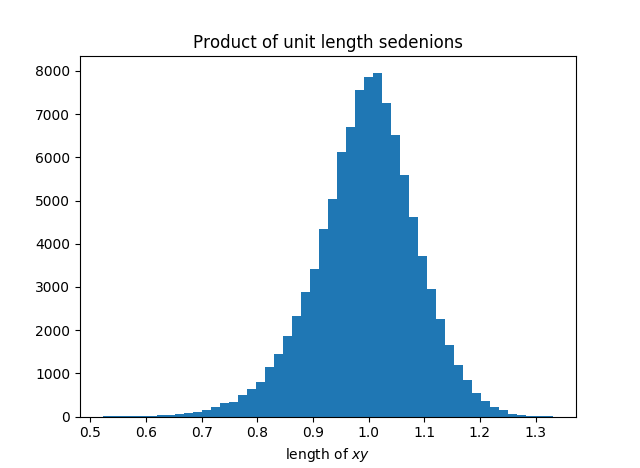
I thought that sedenions also had this norm property, that the product of unit length vectors has unit length. Apparently not, as I discovered by trying to take the inverse cosine of a number larger than 1. So what is the distribution of lengths that come from multiplying two sedenions of length 1? Apparently the mean is near 1, and here’s a histogram.