Empirically testing the Chowla conjecture

Terry Tao’s most recent blog post looks at the Chowla conjecture theoretically. This post looks at the same conjecture empirically using Python. (Which is much easier!)

The Liouville function λ(n) is (-1)Ω(n) where Ω(n) is the number of prime factors of n counted with multiplicity. So, for example, Ω(9) = 2 because even though 9 has only one distinct prime factor, that factor counts twice.

Given some set of k strides h1, h2, …, hk, define

f(n) = λ(n + h1) λ(n + h1) … λ(n + hk).

The Chowla conjecture says that the average of the first N values of f(n) tends to zero as N goes to infinity. This has been proven for k = 1 but not for larger k.

If f(n) acts like a Bernoulli random variable, our experiments might increase our confidence in the conjecture, but they wouldn’t prove anything. Unexpected results wouldn’t prove anything either, but a departure from random behavior might help find a counterexample if the conjecture is false.

We’re going to be evaluating the Liouville function repeatedly at the same arguments, so it will save some compute time if we tabulate its values. This will also let us use some compact Python notation to average f. We’ll need to tabulate the function up to Nhk.

In the code below, maxstride is an upper bound on the strides hk we may look at. SymPy has a function primeomega that calculates Ω(n) so we might as well use it. If you wanted to use a very large value of N, you might want to fill the array of Liouville function values using a more direct approach that avoids all the factoring implicit in calls to primeomega.

    from sympy import primeomega
    from numpy import empty

    N = 10000
    maxstride = 100

    liouville = empty(N + maxstride)
    liouville[0] = 1
    for n in range(1, len(liouville)):
        liouville[n] = (-1)**primeomega(n)

The following code looks at the Chowla conjecture for h1 = 0 and h2 ranging over 1, 2, …, 99.

    average = empty(maxstride-1)
    for s in range(1, maxstride):
        average[s-1] = (liouville[0:N] * liouville[s:N+s]).sum()/N

If the Liouville function is distributed like a random variable taking on -1 and 1 with equal probability, we’d expect the averages to vary like samples form a normal distribution with mean 0 and variance 1/(2N).

    print(average.mean())
    print(average.std())
    print( (2*N)**-0.5 )

This returns

    0.00141
    0.00851
    0.00707

and so the means are indeed near zero, and the standard deviation of the samples is about what we’d expect.

What if we replace Ω(n), the number of prime factors with multiplicity, with ω(n), the number of distinct prime factors? The averages above are still small, but the sample variance is about twice as big as before. I’ve seen this pattern with several different large values of N, so I suspect there’s something going on here.

(I didn’t see a function in SymPy corresponding to ω(n), but you can create your own with len(factorint(n)).

Time series analysis vs DSP terminology

Time series analysis and digital signal processing are closely related. Unfortunately, the two fields use different terms to refer to the same things.

Suppose you have a sequence of inputs x[n] and a sequence of outputs y[n] for integers n.

Moving average / FIR

If each output depends on a linear combination of a finite number of previous inputs

y[n] = b0 x[n] + b1 x[n−1] + … + bq x[nq]

then time series analysis would call this a moving average (MA) model of order q, provided b0 = 1. Note that this might not really be an average, i.e. the b‘s are not necessarily positive and don’t necessarily sum to 1.

Digital signal processing would call this a finite impulse response (FIR) filter of order q.

Autoregressive / IIR

If each output depends on a linear combination of a finite number of previous outputs

y[n] = a1 y[n −1] + … + ap y[np]

then time series analysis would call this an autoregressive (AR) model of order p.

Digital signal processing would call this an infinite impulse response (IIR) filter of order p. 

Sometimes you’ll see the opposite sign convention on the a‘s.

ARMA / IIR

If each output depends on a linear combination of a finite number of previous inputs and outputs

y[n] = b0 x[n] + b1 x[n-1] + … + bq x[nq] + a1 y[n − 1] + … + ap y[np]

then time series analysis would call this an autoregressive moving average (ARMA) model of order (pq), i.e. p AR terms and q MA terms.

Digital signal processing would call this an infinite impulse response (IIR) filter with q feedforward coefficients and p feedback coefficients. Also, as above, you may see the opposite sign convention on the a‘s.

ARMA notation

Box and Jenkins use a‘s for input and z‘s for output. We’ll stick with x‘s and y’s to make the comparison to DSP easier.

Using the backward shift operator B that takes a sample at n to the sample at n-1, the ARMA system can be written

φ(B) y[n] = θ(B) x[n]

where φ and θ are polynomials

φ(B) = 1 − φ1B − φ2B² − … φpBp

and

θ(B) = 1 − θ1B − θ2B² − … θqBq.

System function notation

In DSP, filters are described by their system function, the z-transform of the impulse response. In this notation (as in Oppenheim and Shafer, for example) we have

H(z) = \frac{\sum_{k=0}^q b_k z^{-k}}{1 - \sum_{k=1}^p a_k z^{-k}}

The φk in Box and Jenkins correspond to the ak in Oppenheim and Schafer. The θk correspond to the (negative) bk.

The system function H(z) corresponds to θ(1/z) / φ(1/z).

Related

DSP and time series consulting


Applying probability to non-random things

Probability has surprising uses, including applications to things that absolutely are not random. I’ve touched on this a few times. For example, I’ve commented on how arguments about whether something is really random are often moot: Random is as random does.

This post will take non-random uses for probability in a different direction. We’ll start with discussion of probability and end up proving a classical analysis result.

Let p be the probability of success on some experiment and let Xn count the number of successes in n independent trials. The expected value of Xn is np, and so the expected value of Xn/n is p.

Now let be a continuous function on [0, 1] and think about f(Xn/n). As n increases, the distribution of Xn/n clusters more and more tightly around p, and so f(Xn/n) clusters more and more around f(p).

Let’s illustrate this with a simulation. Let p = 0.6, n = 100, and let f(x) = cos(x).

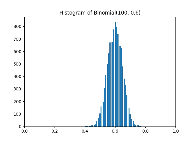
Here’s a histogram of random samples from Xn/n.

Histogram of samples from Bin(100, 0.6)

And here’s a histogram of random samples from f(Xn/n). Note that it’s centered near cos(p) = 0.825.

Histogram of samples from cos( Bin(100, 0.6) )


As n gets large, the expected value of f(Xn/n) converges to f(p). (You could make all this all rigorous, but I’ll leave out the details to focus on the intuitive idea.)

Now write out the expected value of f(Xn/n).

E\left[ f\left(\frac{X_n}{n} \right ) \right ] = \sum_{k=0}^n f\left(\frac{k}{n} \right ) {n \choose k} p^k(1-p)^{n-k}

Up to this point we’ve thought of p as a fixed probability, and we’ve arrived at an approximation result guided by probabilistic thinking. But the expression above is approximately f(p) regardless of how we think of it. So now let’s think of p varying over the interval [0, 1].

E[ f(Xn/n) ] is an nth degree polynomial in p that is close to f(p). In fact, as n goes to infinity, E[ f(Xn/n) ] converges uniformly to f(p).

So for an arbitrary continuous function f, we’ve constructed a sequence of polynomials that converge uniformly to f. In other words, we’ve proved the Weierstrass approximation theorem! The Weierstrass approximation theorem says that there exists a sequence of polynomials converging to any continuous function f on a bounded interval, and we’ve explicitly constructed such a sequence. The polynomials E[ f(Xn/n) ] are known as the Bernstein polynomials associated with f.

This is one of my favorite proofs. When I saw this in college, it felt like the professor was pulling a rabbit out of a hat. We’re talking about probability when all of a sudden, out pops a result that has nothing to do with randomness.

Now let’s see an example of the Bernstein polynomials approximating a continuous function. Again we’ll let f(x) = cos(x). If we plot the Bernstein polynomials and cosine on the same plot, the approximation is good enough that it’s hard to see what’s what. So instead we’ll plot the differences, cosine minus the Bernstein approximations.

Error in approximating cosine by Bernstein polynomials

As the degree of the Bernstein polynomials increase, the error decreases. Also, note the vertical scale. Cosine of zero is 1, and so the errors here are small relative to the size of the function being approximated.

Something that bothers me about deep neural nets

Overfitting happens when a model does too good a job of matching a particular data set and so does a poor job on new data. The way traditional statistical models address the danger of overfitting is to limit the number of parameters. For example, you might fit a straight line (two parameters) to 100 data points, rather than using a 99-degree polynomial that could match the input data exactly and probably do a terrible job on new data. You find the best fit you can to a model that doesn’t have enough flexibility to match the data too closely.

Deep neural networks have enough parameters to overfit the data, but there are various strategies to keep this from happening. A common way to avoid overfitting is to deliberately do a mediocre job of fitting the model.

When it works well, the shortcomings of the optimization procedure yield a solution that differs from the optimal solution in a beneficial way. But the solution could fail to be useful in several ways. It might be too far from optimal, or deviate from the optimal solution in an unhelpful way, or the optimization method might accidentally do too good a job.

It a nutshell, the disturbing thing is that you have a negative criteria for what constitutes a good solution: one that’s not too close to optimal. But there are a lot of ways to not be too close to optimal. In practice, you experiment until you find an optimally suboptimal solution, i.e. the intentionally suboptimal fit that performs the best in validation.


Toxic pairs, re-identification, and information theory

Database fields can combine in subtle ways. For example, nationality is not usually enough to identify anyone. Neither is religion. But the combination of nationality and religion can be surprisingly informative.

Information content of nationality

How much information is contained in nationality? That depends on exactly how you define nations versus territories etc., but for this blog post I’ll take this Wikipedia table for my raw data. You can calculate that nationality has entropy of 5.26 bits. That is, on average, nationality is slightly more informative than asking five independent yes/no questions. (See this post for how to calculate information content.)

Entropy measures expected information content. Knowing that someone is from India (population 1.3 billion) carries only 2.50 bits of information. Knowing that someone is from Vatican City (population 800) carries 23.16 bits of information.

One way to reduce the re-identification risk of PII (personally identifiable information) such as nationality is to combine small categories. Suppose we lump all countries with a population under one million into “other.” Then we go from 240 categories down to 160. This hardly makes any difference to the entropy: it drops from 5.26 bits to 5.25 bits. But the information content for the smallest country on the list is now 8.80 bits rather than 23.16.

Information content of religion

What about religion? This is also subtle to define, but again I’ll use Wikipedia for my data. Using these numbers, we get an entropy of 2.65 bits. The largest religion, Christianity, has an information content 1.67 bits. The smallest religion on the list, Rastafari, has an information content of 13.29 bits.

Joint information content

So if nationality carries 5.25 bits of information and religion 2.65 bits, how much information does the combination of nationality and religion carry? At least 5.25 bits, but no more than 5.25 + 2.65 = 7.9 bits on average. For two random variables X and Y, the joint entropy H(X, Y) satisfies

max( H(X), H(Y) ) ≤ H(X, Y) ≤ H(X) + H(Y)

where H(X) and H(Y) are the entropy of X and Y respectively.

Computing the joint entropy exactly would require getting into the joint distribution of nationality and religion. I’d rather not get into this calculation in detail, except to discuss possible toxic pairs. On average, the information content of the combination of nationality and religion is no more than the sum of the information content of each separately. But particular combinations can be highly informative.

For example, there are not a lot of Jews living in predominantly Muslim countries. According to one source, there are at least five Jews living in Iraq. Other sources put the estimate as “less than 10.” (There are zero Jews living in Libya.)

Knowing that someone is a Christian living in Mexico, for example, would not be highly informative. But knowing someone is a Jew living in Iraq would be extremely informative.

More information

Cellular automata with random initial conditions

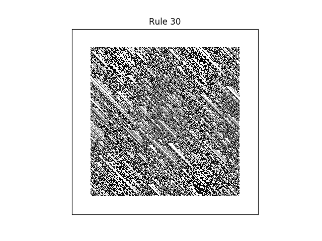
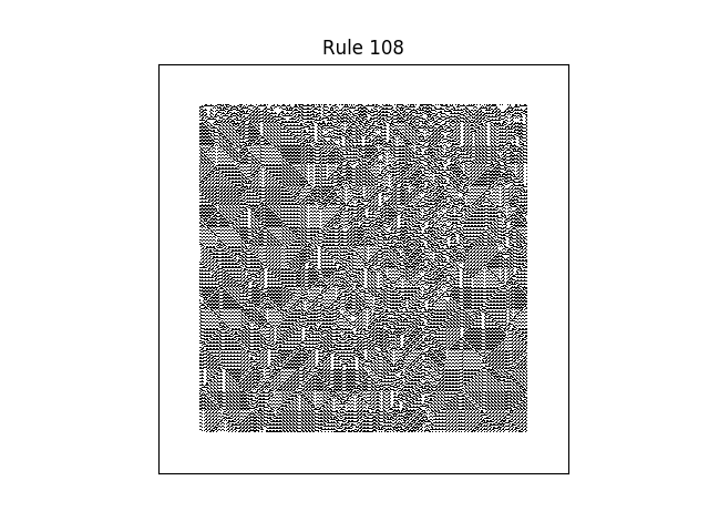
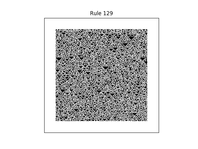
The previous post looked at a particular cellular automaton, the so-called Rule 90. When started with a single pixel turned on, it draws a Sierpinski triangle. With random starting pixels, it draws a semi-random pattern that retains features like the Sierpinski triangle.

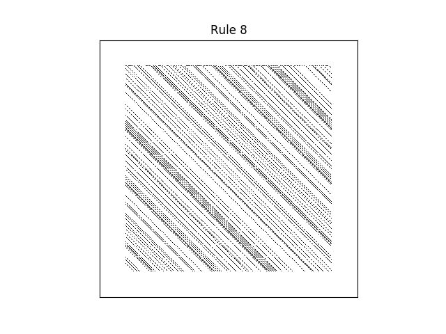
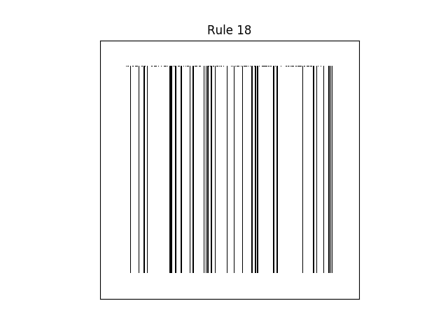
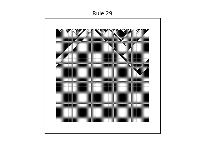
There are only 256 possible elementary cellular automata, so it’s practical to plot them all. I won’t list all the images here—you can find them all here—but I will give a few examples to show the variety of patterns they produce. As in the previous post, we imagine our grid rolled up into a cylinder, i.e. we’ll wrap around if necessary to find pixels diagonally up to the left and right.

rule 8 with random initial conditions
rule 18 with random initial conditions
rule 29 with random initial conditions
rule 30 with random initial conditions
rule 108 with random initial conditions
rule 129 with random initial conditions

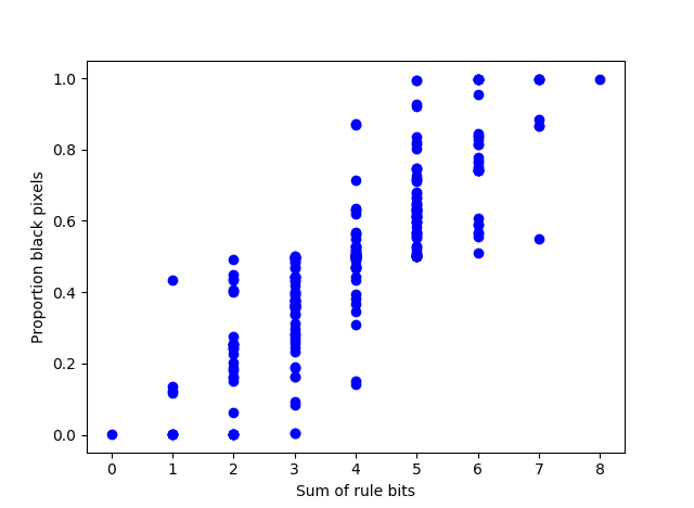
As we discussed in the previous post, the number of a rule comes from what value it assigns to each of eight possible cellular states, turned into a binary number. So it’s plausible that binary numbers with more 1’s correspond to more black pixels. This is roughly true, though the graph below shows that the situation is more complex than that.

automata pixel density as a function of 1 bits in rule

Adding Laplace or Gaussian noise for privacy

pixelated face

In the previous two posts we looked at a randomization scheme for protecting the privacy of a binary response. This post will look briefly at adding noise to continuous or unbounded data. I like to keep the posts here fairly short, but this topic is fairly technical. To keep it short I’ll omit some of the details and give more of an intuitive overview.

Differential privacy

The idea of differential privacy is to guarantee bounds on how much information may be revealed by someone’s participation in a database. These bounds are described by two numbers, ε (epsilon) and δ (delta). We’re primarily interested in the multiplicative bound described by ε. This number is roughly the number of bits of information an analyst might gain regarding an individual. (The multiplicative bound is exp(ε) and so ε, the natural log of the multiplicative bound, would be the information measure, though technically in nats rather than bits since we’re using natural logs rather than logs base 2.)

The δ term is added to the multiplicative bound. Ideally δ is 0, that is, we’d prefer (ε, 0)-differential privacy, but sometimes we have to settle for (ε, δ)-differential privacy. Roughly speaking, the δ term represents the possibility that a few individuals may stand to lose more privacy than the rest, that the multiplicative bound doesn’t apply to everyone. If δ is very small, this risk is very small.

Update: See a detailed introduction to differential privacy here.

Laplace mechanism

The Laplace distribution is also known as the double exponential distribution because its distribution function looks like the exponential distribution function with a copy reflected about the y-axis; these two exponential curves join at the origin to create a sort of circus tent shape. The absolute value of a Laplace random variable is an exponential random variable.

Why are we interested this particular distribution? Because we’re interested in multiplicative bounds, and so it’s not too surprising that exponential distributions might make the calculations work out because of the way the exponential scales multiplicatively.

The Laplace mechanism adds Laplacian-distributed noise to a function. If Δf is the sensitivity of a function f, a measure of how revealing the function might be, then adding Laplace noise with scale Δf/ε preserves (ε 0)-differential privacy.

Technically, Δf is the l1 sensitivity. We need this detail because the results for Gaussian noise involve l2 sensitivity. This is just a matter of whether we measure sensitivity by the l1 (sum of absolute values) norm or the l2 (root sum of squares) norm.

Gaussian mechanism

The Gaussian mechanism protects privacy by adding randomness with a more familiar normal (Gaussian) distribution. Here the results are a little messier. Let ε be strictly between 0 and 1 and pick δ > 0. Then the Gaussian mechanism is (ε, δ)-differentially private provided the scale of the Gaussian noise satisfies

\sigma \geq \sqrt{2 \log(1.25/\delta)}\,\, \frac{\Delta_2 f}{\varepsilon}

It’s not surprising that the l2 norm appears in this context since the normal distribution and l2 norm are closely related. It’s also not surprising that a δ term appears: the Laplace distribution is ideally suited to multiplicative bounds but the normal distribution is not.

Related posts

Quantifying the information content of personal data

It can be surprisingly easy to identify someone from data that’s not directly identifiable. One commonly cited result is that the combination of birth date, zip code, and sex is enough to identify 87% of Americans. This post will look at how to quantify the amount of information contained in such data.

If the answer to a question has probability p, then it contains −log2 p bits of information. Knowing someone’s sex gives you 1 bit of information because −log2(1/2) = 1.

Knowing whether someone can roll their tongue could give you more or less information than knowing their sex. Estimates vary, but say 75% can roll their tongue. Then knowing that someone can roll their tongue gives you 0.415 bits of information, but knowing that they cannot roll their tongue gives you 2 bits of information.

On average, knowing someone’s tongue rolling ability gives you less information than knowing their sex. The average amount of information, or entropy, is

0.75(−log2 0.75) + 0.25(−log2 0.25) = 0.81.

Entropy is maximized when all outcomes are equally likely. But for identifiability, we’re concerned with maximum information as well as average information.

Knowing someone’s zip code gives you a variable amount of information, less for densely populated zip codes and more for sparsely populated zip codes. An average zip code contains about 7,500 people. If we assume a US population of 326,000,000, this means a typical zip code would give us about 15.4 bits of information. (Update: see a more precise calculation here.)

The Safe Harbor provisions of US HIPAA regulations let you use the first three digits of someone’s zip code except when this would represent less than 20,000 people, as it would in several sparsely populated areas. Knowing that an American lives in a region of 20,000 people would give you 14 bits of information about that person.

Birth dates are complicated because age distribution is uneven. Knowing that someone’s birth date was over a century ago is highly informative, much more so than knowing it was a couple decades ago. That’s why the Safe Harbor provisions do not allow including age, much less birth date, for people over 90.

Birthdays are simpler than birth dates. Birthdays are not perfectly evenly distributed throughout the year, but they’re close enough for our purposes. If we ignore leap years, a birthday contains −log2(1/365) or about 8.5 bits of information. If we consider leap years, knowing someone was born on a leap day gives us two extra bits of information.

Independent information is additive. I don’t expect there’s much correlation between sex, geographical region, and birthday, so you could add up the bits from each of these information sources. So if you know someone’s sex, their zip code (assuming 7,500 people), and their birthday (not a leap day), then you have 25 bits of information, which may be enough to identify them.

This post didn’t consider correlated information. For example, suppose you know someone’s zip code and primary language. Those two pieces of information together don’t provide as much information as the sum of the information they provide separately because language and location are correlated. I may discuss the information content of correlated information in a future post. (Update: Here is a post on correlated pairs of data.)

RelatedHIPAA de-identification

Negative correlation introduced by success

Suppose you measure people on two independent attributes, X and Y, and take those for whom X+Y is above some threshold. Then even though X and Y are uncorrelated in the full population, they will be negatively correlated in your sample.

This article gives the following example. Suppose beauty and acting ability were uncorrelated. Knowing how attractive someone is would give you no advantage in guessing their acting ability, and vice versa. Suppose further that successful actors have a combination of beauty and acting ability. Then among successful actors, the beautiful would tend to be poor actors, and the unattractive would tend to be good actors.

Here’s a little Python code to illustrate this. We take two independent attributes, distributed like IQs, i.e. normal with mean 100 and standard deviation 15. As the sum of the two attributes increases, the correlation between the two attributes becomes more negative.

from numpy import arange
from scipy.stats import norm, pearsonr
import matplotlib.pyplot as plt

# Correlation.
# The function pearsonr returns correlation and a p-value.
def corr(x, y):
    return pearsonr(x, y)[0]

x = norm.rvs(100, 15, 10000)
y = norm.rvs(100, 15, 10000)
z = x + y

span = arange(80, 260, 10)
c = [ corr( x[z > low], y[z > low] ) for low in span ]

plt.plot( span, c )
plt.xlabel( "minimum sum" )
plt.ylabel( "correlation coefficient" )
plt.show()

Width of mixture PDFs

Suppose you draw samples from two populations, one of which has a wider probability distribution than the other. How does the width of the distribution of the combined sample vary as you change the proportions of the two populations?

The extremes are easy. If you pick only from one population, then the resulting distribution will be exactly as wide as the distribution of that population. But what about in the middle? If you pick from both populations with equal probability, will the width resulting distribution be approximately the average of the widths of the two populations separately?

To make things more specific, we’ll draw from two populations: Cauchy and normal. With probability η we will sample from a Cauchy distribution with scale γ and with probability (1 − η) we will sample from a normal distribution with scale σ. The resulting combined distribution is a mixture, known in spectroscopy as a pseudo-Voigt distribution. In that field, the Cauchy distribution is usually called the Lorentz distribution.

(Why”pseudo”? A Voigt random variable is the sum of a Cauchy and a normal random variable. Its PDF is a convolution of a Cauchy and a normal PDF. A pseudo-Voigt random variable is the mixture of a Cauchy and a normal random variable. Its PDF is a convex combination of the PDFs of a Cauchy and a normal PDF. In fact, the convex combination coefficients are η and (1-η) mentioned above. Convex combinations are easier to work with than convolutions, at least in some contexts, and the pseudo-Voigt distribution is a convenient approximation to the Voigt distribution.)

We will measure the width of distributions by full width at half maximum (FWHM). In other words, we’ll measure how far apart the two points are where the distribution takes on half of its maximum value.

It’s not hard to calculate that the FWHM for a Cauchy distribution with scale 2γ and the FWHM for a normal distribution with scale σ is 2 √(2 log 2) σ.

If we have a convex combination of Cauchy and normal distributions, we’d expect the FWHM to be at least roughly the same convex combination of the FWHM of the separate distributions, i.e. we’d expect the FWHM of our mixture to be

2ηγ + 2(1 − η)√(2 log 2)σ.

How close is that guess to being correct? It has to be exactly correct when η is 0 or 1, but how well does it do in the middle? Here are a few experiments fixing γ = 1 and varying σ.