Lagrange’s quintic and Descartes’ rule

Do fifth degree polynomial equations come up in applications? Yes, and this post will give an example.

In general the three-body problem, describing the motion of three objects interacting under gravity, does not have a closed-form solution. However, Euler and Lagrange discovered a few special cases that do have closed-form solutions. We will look at Lagrange’s quintic, an equation that came out of Lagrange’s elaboration on Euler’s solution involving three masses moving so that they remain colinear.

Lagrange’s quintic equation is

\begin{align*} (m_1 + m_2)x^5 &+ (3m_1 + 2m_2)x^4 + (3m_1 + m_2)x^3 \\ &- (m_2 + 3m_3)x^2 - (2m_2 + 3m_3)x - (m_2+m_3) = 0 \end{align*}

where m1, m2, and m3 are the masses of the three bodies and x represents the ratio of the distances from the second body to the other two bodies.

Descartes’ rule of signs says that the equation above has exactly one positive root. This is because the signs of the coefficients only change once: the first three coefficients are positive and the next three are negative. Only positive roots are physically meaningful since x represents a ratio of (unsigned) distances, so Laplace’s quintic has a unique meaningful solution. Note that this argument places no restrictions on the relative masses of the three objects.

We can set x = −w and apply Descartes’ rule to the polynomial equation in w. This tells us that the equation has 0, 2, or 4 solutions for positive w, i.e. for negative x. But this doesn’t tell us anything we wouldn’t know from more general principles. Fifth degree polynomials have five roots, and complex roots to equations with real coefficients come in conjugate pairs, so Lagrange equation either has two complex roots (and thus two negative real roots) or four complex roots (and no negative real roots).

Related posts

Artemis lunar orbit

I haven’t been able to find technical details of the orbit of Artemis I, and some of what I’ve found has been contradictory, but here are some back-of-the-envelope calculations based on what I’ve pieced together. If someone sends me better information I can update this post.

Artemis is in a highly eccentric orbit around the moon, coming within 130 km (80 miles) of the moon’s surface at closest pass, and this orbit will take 14 days to complete. The weak link in this data is “14 days.” Surely this number has been rounded for public consumption.

If we assume Artemis is in a Keplerian orbit, i.e. we can ignore the effect of the Earth, then we can calculate the shape of the orbit using the information above. This assumption is questionable because as I understand it the reason for such an eccentric orbit has something to do with Lagrange points, which means the Earth’s gravity matters. Still, I image the effect of Earth’s gravity is a smaller source of error than the lack of accuracy in knowng the period.

Solving for axes

Artemis is orbiting the moon similarly to how the Mars Orbiter Mission orbited Mars. We can use Kepler’s equation for period T to solve for the semi-major axis a of the orbit.

T = 2π √(a³/μ)

Here μ = GM, with G being the gravitational constant and M being the mass of the moon. Now

G = 6.674 × 10⁻¹¹ N m²/kg²

and

M = 7.3459 × 10²² kg.

If we assume T is 14 × 24 × 3600 seconds, then we get

a = 56,640 km

or 35,200 miles. The value of a is rough since the value of T is rough.

Assuming a Keplerian orbit, the moon is at one focus of the orbit, located a distance c from the center of the ellipse. If Artemis is 130 km from the surface of the moon at perilune, and the radius of the moon is 1737 km, then

c = a − (130 + 1737) km = 54,770 km

or 34,000 miles. The semi-minor axis b satisfies

b² = a² − c²

and so

b = 14,422 km

or 8962 miles.

Orbit shape

The eccentricity is c/a = 0.967. As I’ve written about before, eccentricity is hard to interpret intuitively. Aspect ratio is much easier to imaging than eccentricity, and the relation between the two is highly nonlinear.

Assuming everything above, here’s what the orbit would look like. The distances on the axes are in kilometers.

Artemis moon orbit

The orbit is highly eccentric: the center of the orbit is far from the foci of the orbit. But the aspect ratio is about 1/4. The orbit is only about 4 times wider in one direction than the other. It’s obviously an ellipse, but it’s not an extremely thin ellipse.

Lagrange points

In an earlier post I showed how to compute the Lagrange points for the Sun-Earth system. We can use the same equations for the Earth-Moon system.

The equations for the distance r from the Lagrange points L1 and L2 to the moon are

\frac{M_1}{(R\pm r)^2} \pm \frac{M_2}{r^2}=\left(\frac{M_1}{M_1+M_2}R \pm r\right)\frac{M_1+M_2}{R^3}

The equation for L1 corresponds to taking ± as − and the equation for L2 corresponds to taking ± as +. Here M1 and M2 are the masses of the Earth and Moon respectively, and R is the distance between the two bodies.

If we modify the code from the earlier post on Lagrange points we get

L1 = 54784 km
L2 = 60917 km

where L1 is on the near side of the moon and L2 on the far side. We estimated the semi-major axis a to be 56,640 km. This is about 3% larger than the distance from the moon to L1. So the orbit of Artemis passes near or through L1. This assumes the axis of the Artemis orbit is aligned with a line from the moon to Earth, which I believe is at least approximately correct.

Python code to solve Kepler’s equation

The previous post looked at solving Kepler’s equation using Newton’s method. The problem with using Newton’s method is that it may not converge when the eccentricity e is large unless you start very close to the solution. As discussed at the end of that post, John Machin came up with a clever way to start close. His starting point is defined as follow.

\begin{align*} n &= \sqrt{5 + \sqrt{16 + \frac{9}{e}}} \\ M &= n \left((1-e)s + \frac{e(n^2 - 1) + 1}{6}s^3 \right) \\ x_0 &= n \arcsin s \end{align*}

The variable s is implicitly defined as the root of a cubic polynomial. This could be messy. Maybe there are three real roots and we have to decide which one to use. Fortunately this isn’t the case.

The discriminant of our cubic equation is negative, so there is only one real root. And because our cubic equation for s has no s² term the expression for the root isn’t too complicated.

Here’s Python code to solve Kepler’s equation using Newton’s method with Machin’s starting point.

    from numpy import sqrt, cbrt, pi, sin, cos, arcsin, random
    
    # This will solve the special form of the cubic we need.
    def solve_cubic(a, c, d):
        assert(a > 0 and c > 0)
        p = c/a
        q = d/a
        k = sqrt( q**2/4 + p**3/27 )
        return cbrt(-q/2 - k) + cbrt(-q/2 + k)
    
    # Machin's starting point for Newton's method
    # See johndcook.com/blog/2022/11/01/kepler-newton/
    def machin(e, M):
        n = sqrt(5 + sqrt(16 + 9/e))
        a = n*(e*(n**2 - 1)+1)/6
        c = n*(1-e)
        d = -M
        s = solve_cubic(a, c, d)
        return n*arcsin(s)    
    
    def solve_kepler(e, M):
        "Find E such that M = E - e sin E."
        assert(0 <= e < 1)
        assert(0 <= M <= pi) 
        f = lambda E: E - e*sin(E) - M 
        E = machin(e, M) 
        tolerance = 1e-10 

        # Newton's method 
        while (abs(f(E)) > tolerance):
            E -= f(E)/(1 - e*cos(E))
        return E

To test this code, we’ll generate a million random values of e and M, solve for the corresponding value of E, and verify that the solution satisfies Kepler’s equation.

    random.seed(20221102)
    N = 1_000_000
    e = random.random(N)
    M = random.random(N)*pi
    for i in range(N):
        E = solve_kepler(e[i], M[i])
        k = E - e[i]*sin(E) - M[i]
        assert(abs(k) < 1e-10)
    print("Done")

All tests pass.

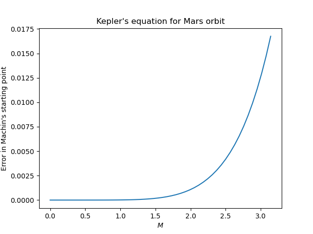
Machin’s starting point is very good, and could make an adequate solution on its own if e is not very large and if you don’t need a great deal of accuracy. Let’s illustrate by solving Kepler’s equation for the orbit of Mars with eccentricity e = 0.09341.

Error in Machin's starting guess as a function of M

Here the maximum error is 0.01675 radians and the average error is 0.002486 radians. The error is especially small for small values of M. When M = 1, the error is only 1.302 × 10⁻⁵ radians.

Solving Kepler’s equation with Newton’s method

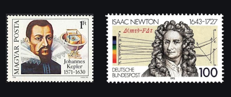
Postage stamps featuring Kepler and Newton

In the introduction to his book Solving Kepler’s Equation Over Three Centuries, Peter Colwell says

In virtually every decade from 1650 to the present there have appeared papers devoted to the Kepler problem and its solution.

This is remarkable because Kepler’s equation isn’t that hard to solve. It cannot be solved in closed form using elementary functions, but it can be solved in many other ways, enough ways for Peter Colwell to write a survey about. One way to find a solution is simply to guess a solution, stick it back in, and iterate. More on that here.

Researchers keep writing about Kepler’s equation, not because it’s hard, but because it’s important. It’s so important that a slightly more efficient solution is significant. Even today with enormous computing resources at our disposal, people are still looking for more efficient solutions. Here’s one that was published last year.

Kepler’s equation

What is Kepler’s equation, and why is it so important?

Kepler’s problem is to solve

M = E - e \sin E

for E, given M and e, assuming 0 ≤ M ≤ π and 0 < e < 1.

This equation is important because it essentially tells us how to locate an object in an elliptical orbit. M is mean anomaly, e is eccentricity, and E is eccentric anomaly. Mean anomaly is essentially time. Eccentric anomaly is not exactly the position of the orbiting object, but the position can be easily derived from E. See these notes on mean anomaly and eccentric anomaly. This is because we’re using our increased computing power to track more objects, such as debris in low earth orbit or things that might impact Earth some day.

Newton’s method

A fairly obvious approach to solving Kepler’s equation is to use Newton’s method. I think Newton himself applied his eponymous method to this equation.

Newton’s method is very efficient when it works. As it starts converging, the number of correct decimal places doubles on each iteration. The problem is, however, that it may not converge. When I taught numerical analysis at Vanderbilt, I used a textbook that quoted this nursery rhyme at the beginning of the chapter on Newton’s method.

There was a little girl who had a little curl
Right in the middle of her forehead.
When she was good she was very, very good
But when she was bad she was horrid.

To this day I think of that rhyme every time I use Newton’s method. When Newton’s method is good, it is very, very good, converging quadratically. When it is bad, it can be horrid, pushing you far from the root, and pushing you further away with each iteration. Finding exactly where Newton’s method converges or diverges can be difficult, and the result can be quite complicated. Some fractals are made precisely by separating converging and diverging points.

Newton’s method solves f(x) = 0 by starting with an initial guess x0 an iteratively applies

x_{n+1} = x_n - \frac{f(x_n)}{f'(x_n)}

Notice that

A sufficient condition for Newton’s method to converge is for x0 to belong to a disk around the root where

\left| \frac{f(x)f''(x)}{f'(x)^2}\right| < 1

throughout the disk.

In our case f is the function

f(x; e, M) = x - e \sin(x) - M

where I’ve used x instead of E because Mathematica reserves E for the base of natural logarithms. To see whether the sufficient condition for convergence given above applies, let’s define

g(x; e, M) = \left| \frac{e(x - e \sin x - M) \sin x}{(1 - e\cos x)^2} \right|

Notice that the denominator goes to 0 as e approaches 1, so we should expect difficulty as e increases. That is, we expect Newton’s method might fail for objects in a highly elliptical orbit. However, we are looking at a sufficient condition, not a necessary condition. As I noted here, I used Newton’s method to solve Kepler’s equation for a highly eccentric orbit, hoping for the best, and it worked.

Starting guess

Newton’s method requires a starting guess. Suppose we start by setting E = M. How bad can that guess be? We can find out using Lagrange multipliers. We want to maximize

(E-M)^2

subject to the constraint that E and E satisfy Kepler’s equation. (We square the difference to get a differentiable objective function to maximize. Minimizing the squared difference minimizes the absolute difference.)

Lagrange’s theorem tells us

\begin{pmatrix} 2x \\ -2M\end{pmatrix} = \lambda \begin{pmatrix} 1 - e \cos x \\ -1\end{pmatrix}

and so λ = 2M and

2x = 2M(1 - e\cos x)

We can conclude that

|x - M| \leq \frac{|e \cos x|}{2} \leq \frac{e}{2} \leq \frac{1}{2}

This says that an initial guess of M is never further than a distance of 1/2 from the solution x, and its even closer when the eccentricity e is small.

If e is less than 0.55 then Newton’s method will converge. We can verify this in Mathematica with

    NMaximize[{g[x, e, M], 0 < e < 0.55, 0 <= M <= Pi, 
        Abs[M - x] < 0.5}, {x, e, M}]

which returns a maximum value of 0.93. The maximum value is an increasing function of the upper bound on e, so converting for e = 0.55 implies converging for e < 0.55. On the other hand, we get a maximum of 1.18 when we let e be as large as 0.60. This doesn’t mean Newton’s method won’t converge, but it means our sufficient condition cannot guarantee that it will converge.

A better starting point

John Machin (1686–1751) came up with a very clever, though mysterious, starting point for solving Kepler’s equation with Newton’s method. Machin didn’t publish his derivation, though later someone was able to reverse engineer how Machin must have been thinking. His starting point is as follows.

\begin{align*} n &= \sqrt{5 + \sqrt{16 + \frac{9}{e}}} \\ M &= n \left((1-e)s + \frac{e(n^2 - 1) + 1}{6}s^3 \right) \\ x_0 &= n \arcsin s \end{align*}

This produces an adequate starting point for Newton’s method even for values of e very close to 1.

Notice that you have to solve a cubic equation to find s. That’s messy in general, but it works out cleanly in our case. See the next post for a Python implementation of Newton’s method starting with Machin’s starting point.

There are simpler starting points that are better than starting with M but not as good as Machin’s method. It may be more efficient to spend less time on the best starting point and more time iterating Newton’s method. On the other hand, if you don’t need much accuracy, and e is not too large, you could use Machin’s starting point as your final value and not use Newton’s method at all. If e < 0.3, as it is for every planet in our solar system, then Machin’s starting point is accurate to 4 decimal places (See Appendix C of Colwell’s book).

Lambert’s theorem

At the start of this series we pointed out that a conic section has five degrees of freedom, and so claims to be able to determine an orbit from less than five numbers must be hiding information somewhere. That is the case with Lambert’s theorem which reportedly determines an orbit from two numbers.

Lambert’s theorem says that the time between two observations of an object in an elliptical orbit can be determined by the sum of the distances to the two observations, the length of the chord connecting the two observations, and the semi-major axis of the ellipse. From this one can determine the equation of the ellipse.

Let r1 be the distance to the first observation and r2 the distance to the second observation, and C the length of the chord between the two observations. We don’t need to know r1 and r2 individually but only their sum r1 + r2. And if we know the angle between the two observations we can use the law of cosines to find C. However we get there, we have two lengths: r1 + r2 and C. We also know a, the length of the semi-major axis. This gives us three lengths.

The observations are taken from the body being orbited, so we implicitly know one of the foci of the ellipse. That’s four pieces of information. The fifth is the mass of the object being orbited.

Lambert’s theorem divides into three cases: elliptic, parabolic, and hyperbolic.

Elliptical orbits

For an object in an elliptic orbit, Lambert’s theorem becomes

\sqrt{\frac{\mu}{a^3}} (t_2 - t_1) = \alpha - \beta - (\sin \alpha - \sin\beta)

where μ is the standard gravitational parameter, equal to GM where G is the gravitational constant and M is the mass of the body orbited. The angles α and β are given by

 \begin{align*} \sin\frac{\alpha}{2} = \frac{1}{2}\left( \frac{r_1 + r_2 + C}{a} \right)^{1/2} \\ \sin\frac{\beta}{2} = \frac{1}{2}\left( \frac{r_1 + r_2 - C}{a} \right)^{1/2} \\ \end{align*}

Hyperbolic orbits

The hyperbolic case is very similar, replacing sine with hyperbolic sine.

\sqrt{\frac{\mu}{a^3}} (t_2 - t_1) = \gamma - \delta - (\sin \gamma - \sin\delta)

where

\begin{align*} \sinh\frac{\gamma}{2} = \frac{1}{2}\left( \frac{r_1 + r_2 + C}{a} \right)^{1/2} \\ \sinh\frac{\delta}{2} = \frac{1}{2}\left( \frac{r_1 + r_2 - C}{a} \right)^{1/2} \\ \end{align*}

Parabolic orbits

The parabolic case was worked out by Newton:

t_2 - t_1 = \frac{1}{6\sqrt{mu}}\left( (r_1 + r_2 + C)^{3/2} - (r_1 + r_2 - C)^{3/2}\right)

Other posts in this series

Source: Adventures in Celestial Mechanics by Victor Szebehely

Gibbs’ method of determining an orbit

Josiah Willard Gibbs

Josiah Willard Gibbs (1839–1903) was prominent American scientist at a time when America had yet to produce many prominent scientists. I first heard of him via Gibbs phenomenon and later by attending one of the Gibbs lectures at an AMS meeting.

Gibbs came up with a method of determining an orbit from three observations. As discussed earlier, a conic section has five degrees of freedom. So how can we determine a conic section, i.e. a two-body problem orbit, from three observations?

Mars Orbiter

As a warm-up to Gibbs’ method, let’s look back at the post on India’s Mars Orbiter Mission. There we determined an orbit by just two observations. What determined the missing three degrees of freedom?

The post on the Mars Orbiter Mission (MOM) didn’t use two arbitrary observations but two very special observations, namely the nearest and furthest approaches of the probe. Because the distances were known relative to Mars, we know the position of one of the foci of the orbit, i.e. the center of mass of Mars. And because the two observations are on opposite sides of the orbit, we know where the other focus is. And because these observations were along the major axis of the ellipse, we know the orientation of the ellipse. All together we know five facts about the orbit.

Gibbsian method

Gibbs method starts with three facts about the orbit, the position of a satellite at three points in its orbit. These are not simply three points on the ellipse but three measurements taken from the body that the satellite is orbiting. That means we know the position of one of the foci, i.e. the body being orbited. Gibbs’ method also assumes we know the mass of body being orbited, so that’s our fifth piece of information.

So with the Mars Orbiter Mission we had two special observations. The “specialness” of these observations provided two more pieces of data, and the fact that the measurements were taken from a focus of the orbit gave us the fifth piece of information.

With Gibbs’ method, we have an extra observation, but none of the observations are special. So we’re up one piece of information from observation but down two pieces of information related to specialness. The missing piece of information is supplied by a physical quantity, the mass of the object orbited.

Radar observation

There is a variation on Gibbs’ method that uses only one observation. It is based on radar observation, not optical observation, and includes the velocity of the object as well as its position. So two partial derivatives, rates of change in two perpendicular directions, replace two of the observations. We still need five bits of information to determine five degrees of freedom.

Preliminary determination

The methods this series of posts use the minimum amount of information algebraically necessary to determine an orbit. In practice, these methods are used for preliminary orbit determination, i.e. they give an approximate result that could be bootstrapped to obtain a more accurate solution.

Under ideal circumstances more further observations would be redundant, but in practice having more observations lets measurement errors cancel each other out to some extent. This observation was a milestone in the development of modern statistics: the problem of determining orbits from multiple observations lead to regression theory.

Notes

You can find the details of how to determine an orbit from three observations in Fundamentals of Astrodynamics by Bate, Mueller, and White. The book also covers determining an orbit from one radar observation with derivatives.

The next post in this series looks at Lambert’s theorem for determining an orbit from two observations (plus three other pieces of information).

Five points determine a conic section

This post is the first in a series looking at determining an orbit. Lambert’s theorem is often summarized by saying you can determine an orbit from two observations. This statement isn’t true without further assumptions, assumptions I plan to make explicit.

A solution to the two-body problem is an orbit given by a conic section, and the general equation of a conic section in the plane is

So conic sections have five degrees of freedom: if you know five out of the six coefficients A, B, C, D, E, and F then the equation above determines the sixth coefficient. And if you know five points on a conic section, there is an elegant way to find an equation of the conic. Given points (xi, yi) for i = 1, …, 5, the following determinant yields an equation for the conic section.

\begin{vmatrix} x^2 & xy & y^2 & x & y & 1 \\ x_1^2 & x_1 y_1 & y_1^2 & x_1 & y_1 & 1 \\ x_2^2 & x_2 y_2 & y_2^2 & x_2 & y_2 & 1 \\ x_3^2 & x_3 y_3 & y_3^2 & x_3 & y_3 & 1 \\ x_4^2 & x_4 y_4 & y_4^2 & x_4 & y_4 & 1 \\ x_5^2 & x_5 y_5 & y_5^2 & x_5 & y_5 & 1 \\ \end{vmatrix} = 0

This means that five observations are enough to determine a conic section, and since Keplerian orbits are conic sections, such an orbit can be determined by five observations. How do we get from five down to two?

Astronomical observations have more context than merely points in a plane. These observations take place over time. So we have not only the positions of objects but their positions at particular times. And we know that the motion of an object in orbit is constrained by Kepler’s laws. In short, we have more data than (x, y) pairs; we have (x, y, t) triples plus physical constraints.

We also have implicit information, and future posts in this series will make this implicit information explicit. For example, suppose you’re planning a trajectory to send a probe to Mars. The path of the probe will essentially be an orbit around the sun. You can determine this orbit by two observations: the position of Earth when the probe leaves and the position of Mars when it arrives. This orbit is not simply an ellipse passing through two points. It is an ellipse with one focus at the sun. I intend to unpack this in a future post, or series of posts, making implicit data explicit.

When I write a series of blog posts, the post don’t always come out consecutively. I expect I’ll write about other topics in between posts in this series.

Update: The next post in the series considers Gibbs’ method of determining an orbit from three observations (plus two other pieces of information). The post after that is about Lambert’s theorem.

Related posts

Elliptical orbit example: Mars Orbiter Mission

This post will look at India’s first interplanetary mission, Mars Orbiter Mission, to illustrate points in recent posts.

Mars Orbiter Mission insignia

As suggested by the logo, the probe had a very eccentric orbit of Mars with periareion 3,812 km and apoareion 80,384 km. We can derive everything else from these numbers. [1]

Peri-what?! As mentioned in footnote 2 of this post the nearest and furthest points of a satellite’s orbit go by various names depending on what the satellite is orbiting. The terms perigee and apogee for Earth satellites are more familiar; the terms periareion and apoareion are the Martian counterparts. The names for the closest and furthest approaches of satellites of Jupiter would be perijove and apojove. The “areion” suffix refers to Ares, the Greek name for Mars.

So the Mars Orbiter Mission (MOM) was much closer to Mars on its nearest approach than on the opposite side of its orbit, 21 times closer. That means its tangential velocity was 21 times faster at periareion than at apoareion [2].

The orbit was an ellipse with major axis 3,812 km + 80,384 km = 84,196 km. The semi-major axis was a = 42,098 km. The center of Mars was a distance c = a – 3,812 km = 38,286 km from the center. The eccentricity was thus e = c/a = 0.909.

Using the equations from this post we find that the aspect ratio of the ellipse was 0.4158.

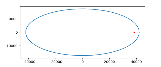
Orbit of Mars Orbiter Mission

Although the deviation of the orbit from circular is substantial, the distance of Mars from the center of the orbit is dramatic. More on this here.

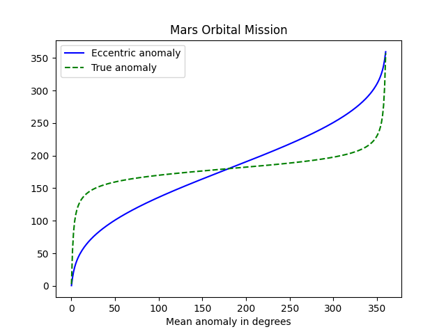
Using the formulas from this post we can plot the mean anomaly, true anomaly, and eccentric anomaly for MOM.

True anomaly and eccentric anomaly of Mars Orbiter Mission

The steep lines on the far left and far right show how quickly the probe is moving at nearest approach to the planet. The true anomaly is the angle to the satellite based at Mars, and this angle changes very rapidly when the probe is near the planet. Eccentric anomaly is measured from the center of the orbit and so it does not change as quickly.

The period along with either the true anomaly or eccentric anomaly is enough to know the position of the satellite at all times. We can determine the period of a satellite from Kepler’s laws:

T = 2π √(a³/μ)

where μ = GM, with G being the gravitational constant and M being the mass of Mars. Now G = 6.674 × 10⁻¹¹ N m²/kg² and M = 6.417 × 10²³ kg. We’ll need to multiply a by 1,000 to work in units of meters. This gives us a period of 262,242 seconds or about 73 hours.

***

[1] My understanding is that while perigee and apogee are measured as altitude from the Earth’s surface, peri[planet] and apo[planet] are conventionally measured from the center of the planet for other planets. That’s how I’m using the terms here. When I first wrote this post, I used a value of periapeion from Wikipedia which was less than the radius of Mars and hence impossible. In retrospect the Wikipedia article was reporting an altitude.

[2] For objects in elliptical orbits, vperi / vapo = rapo / rperi. This follows from Kepler’s law that the vector from a planet to its satellite sweeps out equal area in equal time.

Mean anomaly, true anomaly, and eccentric anomaly

Orbital mechanics has a lot of arcane terminology because it has been studied for centuries. V. I. Arnold said that orbital mechanics was one of the three main sources of modern mathematics.

Mean anomaly, true anomaly, and eccentric anomaly are three ways of describing where an object is in its orbit. All would be the same if planets moved in circular orbits. And since planets nearly do move in circular orbits [1], at least in our solar system, these three anomalies will be similar. We will demonstrate this with plots.

Mean anomaly

Suppose a planet orbiting a star has period T, i.e. it takes time T for the planet to complete one orbit. Let t0 be the time when the planet was closest to the star, i.e. the time since the planet passed through periapsis [2]. Let t be the current time. Then the mean anomaly M is simply

M = 2π(tt0) / T

if you’re working in radians. Change 2π to 360° if you’re working in degrees.

True anomaly

The true anomaly f is the angle with vertex at the star and sides running from the star to periapsis and from the star to the planet. (I don’t know why true anomaly is denoted f. I suppose t and T were taken.)

Eccentric anomaly

The eccentric anomaly E is sorta like the true anomaly, but with the vertex at the center of the elliptical orbit rather than at the star. I say sorta because that’s not quite right.

The eccentric anomaly is an angle with vertex at the center of the elliptical orbit. (The star is not at the center because elliptical orbits are eccentric, literally off-center.) One side does run along the major axis as with the true anomaly, but the other side doesn’t extend from the center to the planet but rather from the center to a projection of the planet’s orbit onto a circle.

Imagine an elliptical orbit in the plane, centered at the origin, with major axis along the x-axis. Now draw a circle around the ellipse with radius equal to the semi-major axis of the ellipse. So the circle touches the ellipse on the two ends, apsis and periapsis, but otherwise extends above and below the ellipse. Take a point P in the orbit and push it out vertically to a point P‘ on the circumscribed circle. That is, keep the x coordinate of P the same, but push the y coordinate up if it’s positive, or down if it’s negative, to get a point on the circle.

Equations

Kepler’s equation relates mean anomaly and eccentric anomaly:

M = Ee sin E

where M is the mean anomaly, E is the eccentric anomaly, and e is the eccentricity of the orbit. So when e is small, M is approximately equal to E.

True anomaly f is related to eccentric anomaly by

f = E + 2 arctan( β sin E / (1 − β cos E) )

where

β = e / (1 + √(1 − e²)).

I’ve written about Kepler’s equation a couple times. Here is a post about a simple way to solve Kepler’s equation for E given M, and here is a post about more efficient ways to solve Kepler’s equation.

Examples

Let’s make some plots comparing mean anomaly, eccentric anomaly, and true anomaly. Mean anomaly is proportional to time, so we’ll use it as our independent variable. Eccentric anomaly and true anomaly are roughly equal to mean anomaly, so we’ll plot the difference between these anomaly and mean anomaly.

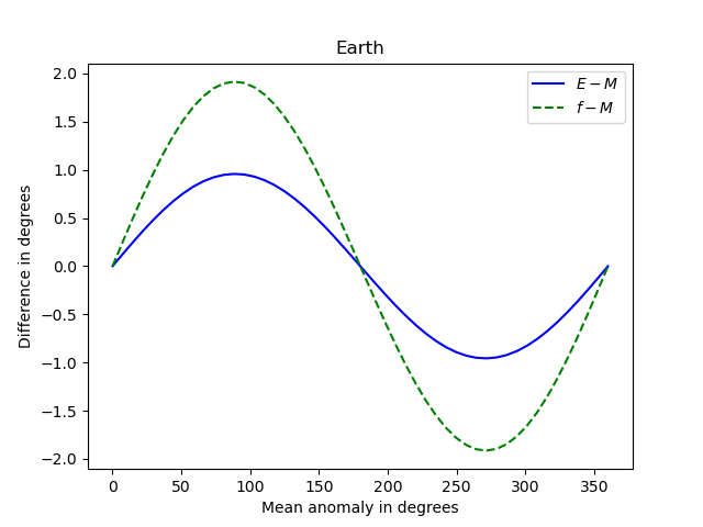
Here’s what we get for Earth, e = 0.01671.

Note that the three anomalies never differ by more than 2 degrees.

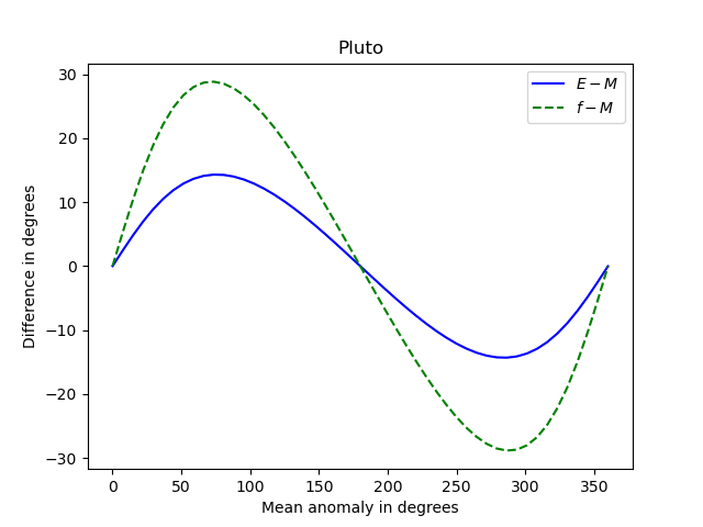
And here’s what we get for Pluto, e = 0.25.

Now the differences between the anomalies is about 15 times greater. The shapes of the curves are roughly the same, but the curves for Earth are more symmetric about their peak and their trough than the corresponding curves for Pluto.

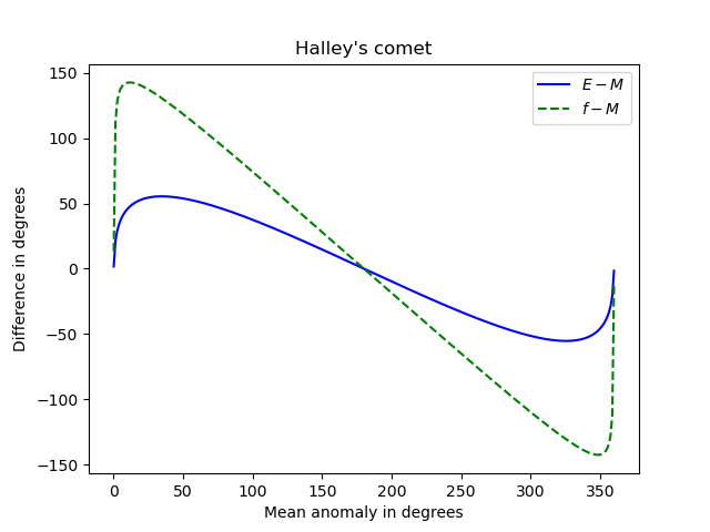
And here’s an extreme example: Halley’s comet. Its orbit has very high eccentricity, e = 0.967.

Newton’s method

I used Newton’s method to solve Kepler’s equation when making the plots above, using the mean anomaly as the initial guess when solving for the eccentric anomaly. I thought I might run into problems with high eccentricity, but everything worked smoothly, even for Halley’s comet. I suppose the basin of attraction for Newton’s method applied to Kepler’s equation is large, at least large enough to include mean anomaly as a starting point.

I didn’t even supply the root-finding method with a derivative functon. I used scipy.optimize.newton with just the function and starting point as arguments, letting the routine construct its own approximate derivative.

Notes

[1] The planets in our solar system move in very nearly circular orbits as explained here. The dwarf planet Pluto has a rather eccentric orbit (e = 0.25) and yet its orbit isn’t far from circular. However, the center of its orbit is far from the sun, as explained here.

[2] This point goes by many names in different contexts. The generic term for this point is called periapsis. For a satellite orbiting the earth it’s called perigee. For an object orbiting our sun it’s called perihelion. For an object orbiting our moon it’s called perilune. …

Cryptography, hydrodynamics, and celestial mechanics

V. I. Arnold

Last night I was reading a paper by the late Russian mathematician V. I. Arnold “Polymathematics: is mathematics a single science or a set of arts?” and posted a lightly edited extract of it on Twitter. It begins

All mathematics is divided into three parts: cryptography, hydrodynamics, and celestial mechanics.

Arnold is alluding to the opening line to Julius Caesar’s Gallic Wars [1] which suggests he’s being a little playful. The unedited version leaves no doubt that he’s being playful or cynical.

All mathematics is divided into three parts: cryptography (paid for by CIA, KGB and the like), hydrodynamics (supported by manufacturers of atomic submarines), and celestial mechanics (financed by military and other institutions dealing with missiles, such as NASA).

I edited out the parenthetical remarks, in part edit the sentence down to a tweet, but also because when you take out the humor/cynicism he makes a valid if hyperbolic point. He goes on to back this up.

Cryptography has generated number theory, algebraic geometry over finite fields, algebra, combinatorics and computers.

Hydrodynamics has procreated complex analysis, partial differential equations, Lie groups and algebra theory, cohomology theory and scientific computing.

Celestial mechanics is the origin of dynamical systems, linear algebra, topology, variational calculus and symplectic geometry.

Arnold adds a footnote to the comment about cryptography:

The creator of modern algebra, Viète, was the cryptographer of King Henry IV of France.

Of course not all mathematics was motivated by cryptography, hydrodynamics, and celestial mechanics, but an awful lot of it was. And his implicit argument that applied math gives birth to pure math is historically correct. Sometimes pure math gives rise to applied math, but much more often it’s the other way around.

His statements roughly match my own experience. Much of the algebra and number theory that I’ve learned has been motivated by cryptography. I dove into Knuth’s magnum opus, volume 2, because I wanted to implement the RSA algorithm in C++.

I got started in scientific computing in a computational fluid dynamics (CDF) lab. I didn’t work in the lab, but my roommate did, and I went there to use the computers. That’s where I would try my hand at numerical analysis and where I wrote simulation code for my dissertation. My dissertation in partial differential equations was related (very abstractly) to fluid flow in porous media.

I didn’t know anything about celestial mechanics until I sat in on Richard Arenstorf‘s class as a postdoc. So celestial mechanics was not my personal introduction to dynamical systems etc., but Arnold is correct that these fields came out of celestial mechanics.

Related posts

[1] “Gallia est omnis divisa in partes tres.” which translates “Gaul is a whole divided into three parts.”