Someone asked on Math Overflow about the distribution of digits in primes. It seems 0 is the least common digit and 1 the most common digit.

Dan Piponi replies “this is probably just a combination of general properties of sets of numbers with a density similar to the primes and the fact that primes end in 1, 3, 7 or 9” and supports this by showing that “fake primes” have very similar digit distributions as actual primes. He generates the nth fake prime by starting with n log n and generating a nearby random integer ending in 1, 3, 7, or 9.

It seems like this fake prime function could be useful for studying more questions. Here is Dan Piponi’s Mathematica implementation:

    fakePrime[n_] :=
      With[
      {m = n Log[n]},
      10 RandomInteger[{Floor[0.09 m], Floor[0.11 m]}] + 
         RandomChoice[{1, 3, 7, 9}]
    ]

Are there more twin stars or twin primes?

If the twin prime conjecture is true, there are an infinite number of twin primes, and that would settle the question.

We don’t know whether there are infinitely many twin primes, and it’s a little challenging to find any results on how many twin primes we’re sure exist.

According to OEIS, we know there are 808,675,888,577,436 pairs of twin primes less than 10¹⁸.

There are perhaps 10²⁴ stars in the observable universe. If so, there are certainly less than 10²⁴ pairs of binary stars in the observable universe. In our galaxy about 2/3 of stars are isolated and about 1/3 come in pairs (or larger clusters). If that holds in every galaxy, then the number of binary stars is within an order of magnitude of the total number of stars.

Do we know for certain there are at least 10²⁴ twin primes? It doesn’t seem anybody is interested in that question. There is more interest in finding larger and larger twin primes. The largest pair currently know have 388,342 digits.

The Hardy-Littlewood conjecture speculates that π₂(x), the number of twin prime pairs less than x, is asymptotically equal to the following

where C₂ is a constant, the product of (1 − 1/(p − 1)²) over all odd primes. Numerically C₂ = 0.6601618….

When x = 10¹⁸ the right hand side of the Hardy Littlewood conjecture agrees with the actual number to at least six decimal places. If the integral gives an estimate of π₂(x) within an order of magntude of being correct for x up to 10²⁸, then there are more twin primes than twin stars.

It’s interesting that our knowledge of both twin stars and twin primes is empirical, though in different ways. We haven’t counted the number of stars in the universe or, as far as I know, the number of twin primes less than 10²⁸, but we have evidence that gives us reason to believe estimates of both.

I recently stumbled across the identity

while reading [1]. Here ⌊x⌋ is the floor of x, the largest integer not larger than x.

My first thought was that this was hard to believe. Although the floor function is very simple, its interactions with other functions tends to be complicated. I was surprised that such a simple equation was true.

My second thought was that the equation makes sense. For large n the three terms on the left are roughly equal, and so

Not only that, the approximation gets better as n gets larger. So the theorem is at least plausible.

My third thought was that there is something subtle going on here. Why the 8 on the right hand side? It turns out the theorem is false if you replace the 8 with a 9. Equality fails to hold for n = 0, 3, 8, 15, …

There is a difference between saying x ≈ y and saying ⌊x⌋ = ⌊y⌋. The former makes the latter plausible, but it’s not the same. If x and y are very close, but on opposite sides of an integer, then ⌊x⌋ ≠ ⌊y⌋.

In fact, the approximation

is better when a = 9 than when a = 8. Here’s a plot of the approximation errors.

So there’s something clever going on with the selection a = 8.

According to [1], the equation at the top was proposed as a problem in 1988 and a solution was published in 2005. The time span between the proposed theorem and its proof suggests that the proof isn’t trivial, though I have not yet read it.

This is an obscure problem, and so we can’t assume that hundreds of mathematicians were feverishly trying to find a solution for 17 years. On the other hand, if there were a trivial proof it seems someone would have posted it quickly.

[1] Prapanpong Pongsriiam. Analytic Number Theory for Beginners, 2nd edition.. American Mathematical Society 2023

Suppose you select a 100-digit number at random. How many distinct prime factors do you think it would have?

The answer is smaller than you might think: most likely between 5 and 6.

The function ω(n) returns the number of distinct prime factors of n [1]. A theorem of Hardy and Ramanujan says that as N goes to infinity, the average value of ω(n) for positive integers up to N is log log N.

Since log log 10¹⁰⁰ = 5.43…, we’d expect 100-digit numbers to have between 5 and 6 distinct factors.

The above calculation gives the average number of distinct prime factors for all numbers with up to 100 digits. But if we redid the calculation looking at numbers between 10⁹⁹ and 10¹⁰⁰ it would only make a difference in the third decimal place.

Let’s look at a much smaller example where we can tally the values of ω(n), numbers from 2 to 1,000,000.

Most numbers with up to six digits have two or three distinct prime factors, which is consistent with log log 10⁶ ≈ 2.6.

There are 2,285 six-digit numbers that have six distinct prime factors. Because this is out of a million numbers, it corresponds to a bar in the graph above that is barely visible.

There are 8 six-digit number with 7 distinct prime factors and none with more factors.

Hardy’s theorem with Ramanujan established the mean of ω(n) for large numbers. The Erdős–Kac theorem goes further and says roughly that ω(n) is normally distributed with mean and variance log log n. More on this here.

So returning to our example of 100-digit numbers, the Hardy-Ramanujan theorem implies these numbers would have between 5 and 6 prime factors on average, and the Erdős–Kac theorem implies that about 95% of such numbers have 10 or fewer distinct prime factors. The maximum number of distinct prime factors is 54.

Related posts

• Prime factors, phone numbers, and the normal distribution
• Distribution of prime powers

[1] SymPy has a function primeomega, but it does not compute ω(n). Instead, it computes Ω(n), the number of prime factors of n counted with multiplicity. So, for example, ω(12) = 2 but Ω(12) = 3. The SymPy function to compute ω(n) is called primenu.

How are the first digits of primes distributed? Do some digits appear as first digits of primes more often that others? How should we even frame the problem?

There are an infinite number of primes that begin with each digit, so the cardinalities of the sets of primes beginning with each digit are the same. But cardinality isn’t the right tool for the job.

The customary way to (try to) approach problems like this is to pose a question for integers up to N and then let N got to infinity. This is called natural density. But this limit doesn’t always converge, and I don’t believe it converges in our case.

Logarithmic density

An alternative is to compute logarithmic density. This measure exists in cases where natural density does not. And when natural density does exist, logarithmic density may give the same result [1].

The logarithmic density of a sequence A is defined by

We want to know about the relative logarithmic density of primes that start with 1, for example. The relative density of a sequence A relative to a sequence B is defined by

We’d like to know about the logarithmic density of primes that start with 1, 2, 3, …, 9 relative to all primes. The exact value is known [2], and we will get to that shortly, but first let’s try to anticipate the result by empirical calculation.

We want to look at the first million primes, and we could do that by calling the function prime with the integers 1 through 1,000,000. But it is much more efficient to as SymPy to find the millionth prime and then find all primes up to that prime.

    from sympy import prime, primerange
    import numpy as np

    first_digit = lambda n: int(str(n)[0])

    density = np.zeros(10)
    N = 1_000_000
    for x in primerange(prime(N+1)):
        density[0] += 1/x
        density[first_digit(x)] += 1/x
    density /= density[0]

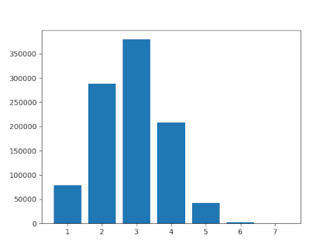
Here’s a histogram of the results.

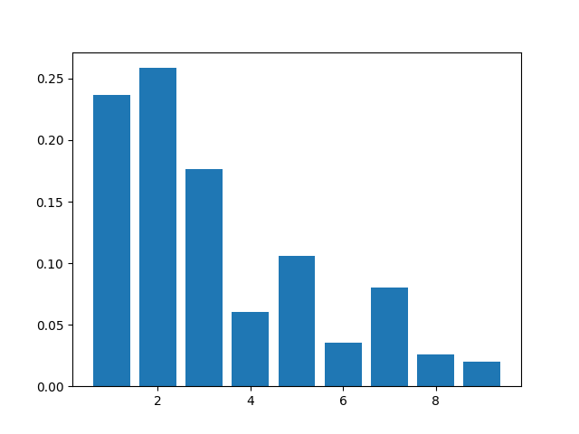
Clearly the distribution is uneven, and in general more primes begin with small digits than large digits. But the distribution is somewhat irregular. That’s how things work with primes: they act something like random numbers, except when they don’t. This sort of amphibious nature, between regularity and irregularity, makes primes interesting.

The limits defining the logarithmic relative density do exist, though the fact that even a million terms doesn’t produce a smooth histogram suggests the convergence is not too rapid.

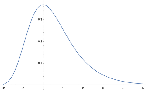
In the limit we get that the density of primes with first digit d is

The densities we’d see in the limit are plotted as follows.

This is exactly the density given by Benford’s law. However, this is not exactly Benford’s law because we are using a different density, logarithmic relative density rather than natural density [3].

Related posts

• Leading digits of factorials
• Alien astronomers and Benford’s law
• Prime numbers and the normal distribution

[1] The Davenport–Erdős theorem says that for some kinds of sequences, if the natural density exists, logarithmic density also exists and will give the same result.

[2] R. E. Whitney. Initial Digits for the Sequence of Primes. The American Mathematical Monthly, Vol. 79, No. 2 (Feb., 1972), pp. 150–152

[3] R. L. Duncan showed that the leading digits of integers satisfy the logarithmic density version of Benford’s law.

If a three-digit number looks like it might be prime, there’s about a 2 in 3 chance that it is.

To be more precise about what it means for a number to “look like a prime,” let’s say that a number is obviously composite if it is divisible by 2, 3, 5, or 11. Then the following Python code quantifies the claim above.

    from sympy import gcd, isprime

    obviously_composite = lambda n: gcd(n, 2*3*5*11) > 1

    primes = 0
    nonobvious = 0

    for n in range(100, 1000):
        if not obviously_composite(n):
            nonobvious += 1
            if isprime(n):
                primes += 1
    print(primes, nonobvious)

This shows that out of 218 numbers that are not obviously composite, 143 are prime.

This is a fairly conservative estimate. It doesn’t consider 707 an obvious composite, for example, even though it’s pretty clear that 707 is divisible by 7. And if you recognize squares like 169, you can add a few more numbers to your list of obviously composite numbers.

The piranha problem says an event cannot be highly correlated with a large number of independent predictors. If you have a lot of strong predictors, they must predict each other, analogous to having too many piranhas in a small body of water: they start to eat each other.

The piranha problem is subtle. It can sound obvious or mysterious, depending on how you state it. You can find several precise formulations of the piranha problem here.

Prime piranhas

An analog of the piranha problem in number theory is easier to grasp. A number N cannot have two prime factors both larger than its square root, nor can it have three prime factors all larger than its cube root. This observation is simple, obvious, and useful.

For example, if N is a three-digit number, then the smallest prime factor of N cannot be larger than 31 unless N is prime. And if N has three prime factors, at least one of these must be less than 10, which means it must be 2, 3, 5, or 7.

There are various tricks for testing divisibility by small primes. The tricks for testing divisibility by 2, 3, and 5 are well known. Tricks for testing divisibility by 7, 11, and 13 are moderately well known. Tests for divisibility by larger primes are more arcane.

Our piranha-like observation about prime factors implies that if you know ways to test divisibility by primes less than p, then you can factor all numbers up to p² and most numbers up to p³. The latter part of this statement is fuzzy, and so we’ll explore it a little further.

How much is “most”?

For a given prime p, what proportion of numbers less than p³ have two factors larger than p? We can find out with the following Python code.

    from sympy import factorint

    def density(p, N = None):
        if not N:
            N = p**3
        count = 0
        for n in range(1, N):
            factors = factorint(n).keys()
            if len([k for k in factors if k > p]) == 2:
                count += 1
        return count/N

The code is a little more general than necessary because in a moment we will like to consider a range that doesn’t necessarily end at p³.

Let’s plot the function above for the primes less than 100.

Short answer: “most” means roughly 90% for primes between 20 and 100.

The results are very similar if we pass in a value of N greater than p³. About 9% of numbers less than 1,000 have two prime factors greater than 10, and about 12% of numbers less than 1,000,000 have two prime factors greater than 100.

Related posts

• Smallest number with a given divisor count
• Conway’s mental factoring algorithm
• How Mr. Bidder calculated logarithms