Haskell analog of Sweave and Pweave

Sweave and Pweave are programs that let you embed R and Python code respectively into LaTeX files. You can display the source code, the result of running the code, or both.

lhs2TeX is roughly the Haskell analog of Sweave and Pweave.  This post takes the sample code I wrote for Sweave and Pweave before and gives a lhs2TeX counterpart.

\documentclass{article}
%include polycode.fmt
%options ghci
\long\def\ignore#1{}
\begin{document}

Invisible code that sets the value of the variable $a$.

\ignore{
\begin{code}
a = 3.14
\end{code}
}

Visible code that sets $b$ and squares it. 

(There doesn't seem to be a way to display the result of a block of code directly. 
Seems you have to save the result and display it explicitly in an eval statement.)

\begin{code}
b = 3.15
c = b*b
\end{code}

$b^2$ = \eval{c}

Calling Haskell inline: $\sqrt{2} = \eval{sqrt 2}$

Recalling the variable $a$ set above: $a$ = \eval{a}.

\end{document}

If you save this code to a file foo.lhs, you can run

lhs2TeX -o foo.tex foo.lhs

to create a LaTeX file foo.tex which you could then compile with pdflatex.

One gotcha that I ran into is that your .lhs file must contain at least one code block, though the code block may be empty. You cannot just have code in \eval statements.

Unlike R and Python, the Haskell language itself has a notion of literate programming. Haskell specifies a format for literate comments. lhs2TeX is a popular tool for processing literate Haskell files but not the only one.

Commutative diagrams in LaTeX

There are numerous packages for creating commutative diagrams in LaTeX. My favorite, based on my limited experience, is Paul Taylor’s package. Another popular package is tikz-cd.

To install Paul Taylor’s package on Windows, I created a directory called localtexmf, set the environment variable TEXINPUTS to its location, and copied diagrams.sty file in that directory.

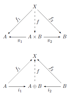
Here are a couple examples, diagrams used in the definition of product and coproduct.

And here’s the LaTeX to produce the diagrams.

\begin{diagram}
& & X & & \\
& \ldTo^{f_1} & \dDashto_f & \rdTo^{f_2} & \\
A & \lTo_{\pi_1} & A\times B & \rTo_{\pi_2} & B \\
\end{diagram}

\begin{diagram}
& & X & & \\
& \ruTo^{f_1} & \uDashto_f & \luTo^{f_2} & \\
A & \rTo_{i_1} & A\oplus B & \lTo_{i_2} & B \\
\end{diagram}

For much more information, see the package page.

RelatedApplied category theory

Unicode to LaTeX

I’ve run across a couple websites that let you enter a LaTeX symbol and get back its Unicode value. But I didn’t find a site that does the reverse, going from Unicode to LaTeX, so I wrote my own.

Unicode / LaTeX Conversion

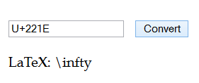
If you enter Unicode, it will return LaTeX. If you enter LaTeX, it will return Unicode. It interprets a string starting with “U+” as a Unicode code point, and a string starting with a backslash as a LaTeX command.

screenshot of www.johndcook.com/unicode_latex.png

For example, the screenshot above shows what happens if you enter U+221E and click “convert.” You could also enter infty and get back U+221E.

However, if you go from Unicode to LaTeX to Unicode, you won’t always end up where you started. There may be multiple Unicode values that map to a single LaTeX symbol. This is because Unicode is semantic and LaTeX is not. For example, Unicode distinguishes between the Greek letter Ω and the symbol Ω for ohms, the unit of electrical resistance, but LaTeX does not.

Automatic delimiter sizes in LaTeX

I recently read a math book in which delimiters never adjusted to the size of their content or the level of nesting. This isn’t unusual in articles, but books usually pay more attention to typography.

Here’s a part of an equation from the book:

\varphi^{-1} (\int \varphi(f+g) \,d\mu)

Larger outer parentheses make the equation much easier to read, especially as part of a complex equation. It’s clear at a glance that the function φ−1 applies to the result of the integral.

\varphi^{-1} \left(\int \varphi(f+g) \,d\mu\right)

The first equation was typeset using

    \varphi^{-1} ( \int \varphi(f+g) \,d\mu )

The latter used left and right to tell LaTeX that the parentheses should grow to match the size of the content between them.

    \varphi^{-1} \left( \int \varphi(f+g) \,d\mu \right)

You can use \left and \right with more delimiters than just parentheses: braces, brackets, ceiling, floor, etc. And the left and right delimiters do not need to match. You could make a half-open interval, for example, with \left( on one side and \right] on the other.

For every \left delimiter there must be a corresponding \right delimiter. However, you can make one of the pair empty by using a period as its mate. For example, you could start an expression with \left[ and end it with \right. which would create a left bracket as tall as the tallest thing between that bracket and the corresponding \right. command. Note that \right. causes nothing to be displayed, not even a period.

The most common example of a delimiter with no mate may be a curly brace on the left with no matching brace on the right. In that case you’d need to open with \left\{. The backslash in front of the brace is necessary to tell LaTeX that you want a literal brace and that you’re not just using the brace for grouping.

Basics of Sweave and Pweave

Sweave is a tool for embedding R code in a LaTeX file. Pweave is an analogous tool for Python. By putting your code in your document rather than the results of running your code somewhere else, results are automatically recomputed when inputs change. This is especially useful with graphs: rather than including an image into your document, you include the code to create the image.

To use either Sweave or Pweave, you create a LaTeX file and include source code inside. A code block begins with <<>>= and ends with @ on a line by itself. By default, code blocks appear in the LaTeX output. You can start a code block with <<echo=FALSE>>= to execute code without echoing its source. In Pweave you can also use <% and %> to mark a code block that executes but does not echo. You might want to do this at the top of a file, for example, for import statements.

Sweave echos code like the R command line, with > for the command prompt. Pweave does not display the Python >>> command line prompt by default, though it will if you use the option term=TRUE in the start of your code block.

In Sweave, you can use Sexpr to inline a little bit of R code. For example, $x = Sexpr{sqrt(2)}$ will produce x = 1.414…. You can also use Sexpr to reference variables defined in previous code blocks. The Pweave analog uses <%= and %>. The previous example would be $x = <%= sqrt(2) %>$.

You can include a figure in Sweave or Pweave by beginning a code block with <<fig=TRUE, echo=FALSE>>= or with echo=TRUE if you want to display the code that produces the figure. With Sweave you don’t need to do anything else with your file. With Pweave you need to add usepackage{graphicx} at the top.

To process an Sweave file foo.Rnw, run Sweave("foo.Rnw") from the R command prompt. To process a Pweave file foo.Pnw, run Pweave -f tex foo.Pnw from the shell. Either way you get a LaTeX file that you can then compile to a PDF.

Here are sample Sweave and Pweave files. First Sweave:

\documentclass{article}
\begin{document}

Invisible code that sets the value of the variable $a$.

<<<echo=FALSE>>=
a <- 3.14
@

Visible code that sets $b$ and squares it.

<<bear, echo=TRUE>>=
b <- 3.15
b*b
@

Calling R inline: $\sqrt{2} = Sexpr{sqrt(2)}$

Recalling the variable $a$ set above: $a = Sexpr{a}$.

Here's a figure:

<<fig=TRUE, echo=FALSE>>=
x <- seq(0, 6*pi, length=200)
plot(x, sin(x))
@

\end{document}

And now Pweave:

\documentclass{article}
\usepackage{graphicx}
\begin{document}

<%
import matplotlib.pyplot as plt
from numpy import pi, linspace, sqrt, sin
%>

Invisible code that sets the value of the variable $a$.

<<echo=FALSE>>=
a = 3.14
@

Visible code that sets $b$ and squares it.

<<term=True>>=
b = 3.15
print b*b
@

Calling Python inline: $\sqrt{2} = <%= sqrt(2) %>$

Recalling the variable $a$ set above: $a = <%= a %>$.

Here's a figure:

<<fig=True, echo=False>>=
x = linspace(0, 6*pi, 200)
plt.plot(x, sin(x))
plt.show()
@

\end{document}

Related links

The paper is too big

In response to the question “Why are default LaTeX margins so big?” Paul Stanley answers

It’s not that the margins are too wide. It’s that the paper is too big!

This sounds flippant, but he gives a compelling argument that paper really is too big for how it is now used.

As is surely by now well-known, the real question is the size of the text block. That is a really important factor in legibility. As others have noted, the optimum line length is broadly somewhere between 60 characters and 75 characters.

Given reasonable sizes of font which are comfortable for reading at the distance we want to read at (roughly 9 to 12 point), there are only so many line lengths that make sense. If you take a book off your shelf, especially a book that you would actually read for a prolonged period of time, and compare it to a LaTeX document in one of the standard classes, you’ll probably notice that the line length is pretty similar.

The real problem is with paper size. As it happens, we have ended up with paper sizes that were never designed or adapted for printing with 10-12 point proportionally spaced type. They were designed for handwriting (which is usually much bigger) or for typewriters. Typewriters produced 10 or 12 characters per inch: so on (say) 8.5 inch wide paper, with 1 inch margins, you had 6.5 inches of type, giving … around 65 to 78 characters: in other words something pretty close to ideal. But if you type in a standard proportionally spaced font (worse, in Times—which is rather condensed because it was designed to be used in narrow columns) at 12 point, you will get about 90 to 100 characters in the line.

He then gives six suggestions for what to do about this. You can see his answer for a full explanation. Here I’ll just summarize his points.

  1. Use smaller paper.
  2. Use long lines of text but extra space between lines.
  3. Use wide margins.
  4. Use margins for notes and illustrations.
  5. Use a two column format.
  6. Use large type.

Given these options, wide margins (as in #3 and #4) sound reasonable.

Separating presentation from content

In the late ’90s I went to a fair number of Microsoft presentations. One presentation would say “The problem with Technology X is that it mixes presentation and content. We’ve introduced Technology Y to make your code cleaner, separating presentation and content.” A few months later I’d be at another presentation that would announce “The problem with Technology Y is that it mixes presentation and content. We’ve introduced Technology Z …” (Does this remind anyone else of The Cat in the Hat Comes Back?)

When I first learned LaTeX, I was told that one of its strengths is that it separates presentation and content. Then a few years later I hear complaints that the problem with LaTeX is that it mingles presentation and content, unlike XHTML. A few years later, guess what? XHTML mixes presentation and content, so we need something else.

I shut down when I hear someone announce that everything before their product was bad because it mixed presentation and content, and now with their solution, presentation and content will be completely separate.

Sometimes one technology really does make a cleaner separation of presentation and content. But at best the separation is relative. LaTeX separates presentation and content more than Word, though not as much as well-written HTML and CSS, maybe. But presentation and content cannot be entirely separated. Nor is there unanimous agreement on what exactly the dividing line is between the two.

Many people don’t want to separate their presentation and content. They don’t understand why this would be desirable, and they’ll fight against anything designed to encourage separation. Maybe they need to learn the advantages, or maybe they’re just doing the best they can to get their job done and they can’t be bothered with long term advantages that may not materialize.

The principle of separating presentation and content is admirable. It really does have advantages, but it’s easier said than done.

Typesetting “C#” in LaTeX

How do you refer to the C# programming language in LaTeX? Simply typing C# doesn’t work because # is a special character in LaTeX. You could type C#. That works, but it looks a little odd. The number sign is too big and too low.

What about using a musical sharp sign, i.e. C$\sharp$? That also looks a little odd. Even though the language is pronounced “C sharp,” it’s usually written with a number sign, not a sharp.

Let’s look at recommended ways of typesetting C++ to see whether that helps. The top answer to this question on TeX Stack Exchange is to define a new command as follows:

\newcommand{\CC}{C\nolinebreak\hspace{-.05em}\raisebox{.4ex}{\tiny\bf +}\nolinebreak\hspace{-.10em}\raisebox{.4ex}{\tiny\bf +}}

This does several things. First, it prevents line breaks between the constituent characters. It also does several things to the plus signs:

  • Draws them in closer
  • Makes them smaller
  • Raises them
  • Makes them bold

The result is what we’re subconsciously accustomed to seeing in print.

Here’s an analogous command for C#.

\newcommand{\CS}{C\nolinebreak\hspace{-.05em}\raisebox{.6ex}{\tiny\bf \#}}

And here’s the output. The number sign is a little too small.

To make a little larger number sign, replace \tiny with \scriptsize.

More LaTeX posts