Monotonic interpolation

Accuracy isn’t everything. Sometimes when you’re approximating a function you care more about matching a function’s qualitative behavior than matching its numerical values.

One example is interpolating monotonic data. Say your data show that increasing input always increases output. It’s likely you want a function that interpolates your data to have the same property and that you might sacrifice some accuracy to assure monotonicity. In a visual application, you might get a distracting wiggle in what should be a smoothly bending curve. In software used to control a physical device, it could lead to unexpected behavior, or even disaster, if an increase in input led to a decrease in output, even if it was a small decrease.

Linear interpolation preserves monotonicity: if in your data increasing x leads to increasing y, the same is true of a linear interpolation to the data. But for higher-order interpolation this isn’t the case. A simple example would be the three points (-1, 1), (2, 4), and (3, 9). The unique quadratic polynomial interpolating these three points is x², which is not monotonic in any interval containing 0. We’d like to have a smoother and more accurate [1] way to interpolate data while still preserving monotonicity.

It’s unlikely that a polynomial interpolating monotone data will be monotone. I suspect that given a set of monotonic data, it’s more likely that a polynomial spline interpolant will be monotone than a polynomial interpolant because the former is more flexible. Formulating this suspicion into a conjecture that could be settled theoretically, or even tested empirically, would be a non-trivial but interesting exercise.

A cubic spline interpolating monotone data is not necessarily monotone. However, there is a way to determine derivative conditions so that a Hermite spline fitting the data will be monotone. Fritsch and Carleson published an algorithm for this in 1980.

Related posts

[1] If the function sampled by your data is smooth, then in general a smooth approximation to the function will be more accurate than a piecewise linear approximation.

Tridiagonal systems, determinants, and natural cubic splines

Tridiagonal matrices

A tridiagonal matrix is a matrix that has nonzero entries only on the main diagonal and on the adjacent off-diagonals. This special structure comes up frequently in applications. For example, the finite difference numerical solution to the heat equation leads to a tridiagonal system. Another application, the one we’ll look at in detail here, is natural cubic splines. And we’ll mention an interesting result with Fibonacci numbers in passing.

Because these matrices have a special structure, the corresponding linear systems are quick and easy to solve. Also, we can find a simple recurrence relation for their determinants.

Determinants

Let’s label the component of a tridiagonal matrix as below

M_n = \left( \begin{array}{lllll} a_1 & b_1 & & & \\ c_1 & a_2 & b_2 & & \\ & c_2 & \ddots & \ddots & \\ & & \ddots & \ddots & b_{n-1} \\ & & & c_{n-1} & a_n \\ \end{array} \right)

where every component not shown is implicitly zero. We can expand the determinant of the matrix above using minors along the last row. This gives a recursive expression for the determinant

d_n = a_n d_{n-1} - c_{n-1} b_{n-1} d_{n-2}

with initial conditions d0 = 1 and d−1 = 0.

Note that if all the a‘s and b‘s are 1 and all the c‘s are −1, then you get the recurrence relation that defines the Fibonacci numbers. That is, the Fibonacci numbers are given by the determinant

F_{n+1} = \left| \begin{array}{rrrrr} 1 & 1 & & & \ldots \\ -1 & 1 & 1 & & \ldots \\ & -1 & \ddots & \ddots & \\ & & \ddots & \ddots & 1 \\ & & & -1 & 1 \\ \end{array} \right|

Natural cubic splines

A cubic spline interpolates a set of data points with piecewise cubic polynomials. There’s a (potentially) different cubic polynomial over each interval between input values, all fitted together so that the resulting function, its derivative, and its second derivative are all continuous.

Suppose you have input points, called knots in this context, t0, t1, … tn and output values y0, y1, … yn. For the spline to interpolate the data, its value at ti must be yi.

A cubic spline then is a set of n cubic polynomials, one for each interval [ti, ti+1]. A cubic polynomial has four coefficients, so we have 4n coefficients in total. At each interior knot, t1 through tn−1, we have four constraints. Both polynomials that meet at ti must take on the value yi at that point, and the two polynomials must have the same first and second derivative at that point. That gives us 4(n − 1) equations. The value of the first polynomial is specified on the left end at t0 the value of the last polynomial is specified at the right end at tn. This gives us 4n − 2 equations in total.

We need two more equations. A clamped cubic spline specifies the derivatives at each end point. The natural cubic spline specifies instead that the second derivatives at each end are zero. What is natural about a natural cubic spline? In a certain sense it is the smoothest curve interpolating the specified points. With these boundary conditions we now have as many constraints as degrees of freedom.

So how would we go about finding the coefficients of each polynomial? Our task will be much easier if we parameterize the polynomials cleverly to start with. Instead of powers of x, we want powers of (xti) and (ti+1x) because these expressions are 0 on different ends of the interval [ti, ti+1]. It turns out we parameterize the spline over the ith interval as

\begin{eqnarray*} S_i(x) &=& \frac{z_{i+1}}{6h_i}(x-t_i)^3 + \frac{z_i}{6h_i}(t_{i+1} - x)^3 \\ && + \left(\frac{y_{i+1}}{h_i} - \frac{h_iz_{i+1}}{6}\right) (x - t_i) \\ && + \left(\frac{y_{i }}{h_i} - \frac{h_iz_i }{6}\right) (t_{i+1} - x) \end{eqnarray*}

where hi = ti+1ti, the length of the ith interval.

This may seem unmotivated, and no doubt it is cleaner than the first thing someone probably tried, but it’s the kind of thing you’re lead to when you try to make the derivation work out smoothly.

The basic form is  powers of (xti) and (ti+1x), each to the first and third powers, for reasons given above. Why the 6’s in the denominators? They’re not strictly necessary, but they cancel out when we take second derivatives. Let’s look at the second derivative.

S_i''(x) = \frac{z_{i+1}(x - t_i)}{h_i} - \frac{z_{i}(t_{i+1} - x)}{h_i}

Note how when we stick in ti the first term is zero and the second is zi, and when we stick in ti+1 the first term is zi+1 and the second is zero.

We can now write down the system of equations for the z‘s. We have z0 = zn from the natural cubic spline condition, and for 1 ≤ in − 1 we have

h_{i-1}z_{i-1} + u_i z_i + h_i z_{i+1} = v_i

where

\begin{eqnarray*}b_i &=& (y_{i+1} - y_i)/h_i \\ u_i &=& 2(h_{i-1} + h_i) \\ v_i &=& 6(b_i - b_{i-1}) \end{eqnarray*}
Note that this is a tridiagonal system because the ith equation only involves z‘s with subscripts i − 1, i, and i + 1.

Because of its tridiagonal structure, these equations can be solved simply and efficiently, much more efficiently than a general system of equations.

Related math posts

Runge phenomena

I’ve mentioned the Runge phenomenon in a couple posts before. Here I’m going to go into a little more detail.

First of all, the “Runge” here is Carl David Tolmé Runge, better known for the Runge-Kutta algorithm for numerically solving differential equations. His name rhymes with cowabunga, not with sponge.

Runge showed that polynomial interpolation at evenly-spaced points can fail spectacularly to converge. His example is the function f(x) = 1/(1 + x²) on the interval [−5, 5], or equivalently, and more convenient here, the function f(x) = 1/(1 + 25x²) on the interval [−1, 1]. Here’s an example with 16 interpolation nodes.

Runge's example

Runge found that in order for interpolation at evenly spaced nodes in [−1, 1] to converge, the function being interpolated needs to be analytic inside a football-shaped [1] region of the complex plane with major axis [−1, 1] on the real axis and minor axis approximately [−0.5255, 0.5255]  on the imaginary axis. For more details, see [2].

The function in Runge’s example has a singularity at 0.2i, which is inside the football. Linear interpolation at evenly spaced points would converge for the function f(x) = 1/(1 + x²) since the singularity at i is outside the football.

Runge's example

For another example, consider the function f(x) = exp(−1/x²) , defined to be 0 at 0. This function is infinitely differentiable but it is not analytic at the origin. With only 16 interpolation points as above, there’s a small indication of trouble at the ends.

Interpolating exp(-1/x^2)

With 28 interpolation points in the plot below, the lack of convergence is clear.

Interpolating exp(-1/x^2)

The problem is not polynomial interpolation per se but polynomial interpolation at evenly-spaced nodes. Interpolation at Chebyshev points converges for the examples here. The location of singularities effects the rate of convergence but not whether the interpolants converge.

RelatedHelp with interpolation

***

[1] American football, that is. The region is like an ellipse but pointy at −1 and 1.

[2] Approximation Theory and Approximation Practice by Lloyd N. Trefethen

Chebyshev interpolation

Fitting a polynomial to a function at more points might not produce a better approximation. This is Faber’s theorem, something I wrote about the other day.

If the function you’re interpolating is smooth, then interpolating at more points may or may not improve the fit of the interpolation, depending on where you put the points. The famous example of Runge shows that interpolating

f(x) = 1 / (1 + x²)

at more points can make the fit worse. When interpolating at 16 evenly spaced points, the behavior is wild at the ends of the interval.

Runge example

Here’s the Python code that produced the plot.

    import matplotlib.pyplot as plt
    from scipy import interpolate, linspace

    def cauchy(x):
        return (1 + x**2)**-1

    n = 16
    x = linspace(-5, 5, n) # points to interpolate at

    y = cauchy(x)
    f = interpolate.BarycentricInterpolator(x, y)

    xnew = linspace(-5, 5, 200) # points to plot at
    ynew = f(xnew)
    plt.plot(x, y, 'o', xnew, ynew, '-')
    plt.show()

However, for smooth functions interpolating at more points does improve the fit if you interpolate at the roots of Chebyshev polynomials. As you interpolate at the roots of higher and higher degree Chebyshev polynomials, the interpolants converge to the function being interpolated. The plot below shows how interpolating at the roots of T16, the 16th Chebyshev polynomial, eliminates the bad behavior at the ends.

Runge example at Chebyshev nodes

To make this plot, we replaced x above with the roots of T16, rescaled from the interval [-1, 1] to the interval [-5, 5] to match the example above.

    x = [cos(pi*(2*k-1)/(2*n)) for k in range(1, n+1)]
    x = 5*array(x)

What if the function we’re interpolating isn’t smooth? If the function has a step discontinuity, we can see Gibbs phenomena, similar to what we saw in the previous post. Here’s the result of interpolating the indicator function of the interval [−1, 1] at 100 Chebyshev points. We get the same “bat ears” as before.

Gibbs phenomena for Chebyshev interpolation

Related: Help with interpolation

Yogi Berra meets Pafnuty Chebyshev

I just got an evaluation copy of The Best Writing on Mathematics 2017. My favorite chapter was Inverse Yogiisms by Lloyd N. Trefethen.

Trefethen gives several famous Yogi Berra quotes and concludes that

Yogiisms are statements that, if taken literally, are meaningless or contradictory or nonsensical or tautological—yet nevertheless convey something true.

An inverse yogiism is the opposite,

[a] statement that is literally true, yet conveys something false.

What a great way to frame a chapter! Now that I’ve heard the phrase, I’m trying to think of inverse yogiisms. Nothing particular has come to mind yet, but I feel like there must be lots of things that fit that description. Trefethen comes up with three inverse yogiisms, and my favorite is the middle one: Faber’s theorem on polynomial interpolation.

Faber’s theorem is a non-convergence result for interpolants of continuous functions. Trefethen quotes several numerical analysis textbooks that comment on Faber’s theorem in a way that implies an overly pessimistic interpretation. Faber’s theorem is true for continuous functions in general, but if the function f  being interpolated is smooth, or even just Lipschitz continuous, the theorem doesn’t hold. In particular, Chebyshev interpolation produces a sequence of polynomials converging to f.

A few years ago I wrote a blog post that shows a famous example due to Carle Runge that if you interpolate f(x) = 1/(1 + x²) over [−5, 5] with evenly spaced nodes, the sequence of interpolating polynomials diverges. In other words, adding more interpolation points makes the fit worse.

Here’s the result of fitting a 16th degree polynomial to f  at evenly spaced nodes.

graph of f(x) and p16(x)

The error near the ends is terrible, though the fit does improve in the middle. If instead of using evenly spaced nodes you use the roots of Chebyshev polynomials, the interpolating polynomials do in fact converge, and converge quickly. If the kth derivative of f has bounded variation, then the error in interpolating f at n points is O(nk).

How to digitize a graph

Suppose you have a graph of a function, but you don’t have an equation for it or the data that produced it. How can you reconstruction the function?

There are a lot of software packages to digitize images. For example, Web Plot Digitizer is one you can use online. Once you have digitized the graph at a few points, you can fit a spline to the points to approximately reconstruct the function. Then as a sanity check, plot your reconstruction to see if it looks like the original. It helps to have the same aspect ratio so you’re not distracted by something that doesn’t matter, and so that differences that do matter are easier to see.

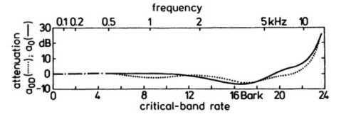
For example, here is a graph from Zwicker and Fastl’s book on psychoacoustics. It contains many graphs with no data or formulas. This particular one gives the logarithmic transmission factor between free field and the peripheral hearing system.

Here’s Python code to reconstruct the functions behind these two curves.

import matplotlib.pyplot as plt
import numpy as np
from scipy import interpolate 

curve_names = ["Free", "Diffuse"]
plot_styles = { "Free" : 'b-', "Diffuse" : 'g:'}

data = {}
for name in curve_names:
    data = np.loadtxt("{}.csv".format(name), delimiter=',')

    x = data[:,0]
    y = data[:,1]
    spline = interpolate.splrep(x, y)
    xnew = np.linspace(0, max(x), 100)
    ynew = interpolate.splev(xnew, spline, der=0)
    plt.plot(xnew, ynew, plot_styles[name])
 
logical_x_range  = 24    # Bark
logical_y_range  = 40    # dB
physical_x_range = 7     # inch
physical_y_range = 1.625 # inch

plt.legend(curve_names, loc=2)
plt.xlabel("critical-band rate")
plt.ylabel("attenuation")
plt.xlim((0, logical_x_range))


plt.axes().set_aspect( 
    (physical_y_range/logical_y_range) / 
    (physical_x_range/logical_x_range) )
ax = plt.gca()
ax.get_xaxis().set_ticks([0, 4, 8, 12, 16, 20, 24])
ax.get_yaxis().set_ticks([-10, 0, 10, 20, 30])

plt.show()

Here’s the reconstructed graph.

Interpolation errors

Say you have a function f(x) and you want to find a polynomial p(x) that agrees with f(x) at several points. Given a set of points

x0, x1, x2, …, xn

you can always find a polynomial of degree n such that p(xi) = f(xi) for i = 0, 1, 2, …, n. It seems reasonable that the more points you pick, the better the interpolating polynomial p(x) will match the function f(x). If the two functions match exactly at a lot of points, they should match well everywhere. Sometimes that’s true and sometimes it’s not.

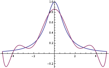
Here is a famous example due to Carle Runge. Let f(x) = 1/(1 + x2) and let pn be the polynomial that interpolates f(x) at n+1 evenly spaced nodes in the interval [−5, 5]. As n becomes larger, the fit becomes worse.

Here’s a graph of f(x) and p9(x). The smooth blue line is f(x) and the wiggly red line is p9(x).

graph of f(x) and p9(x)

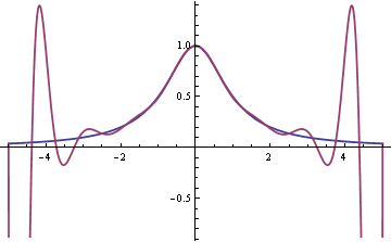
Here’s the analogous graph for p16(x).

graph of f(x) and p16(x)

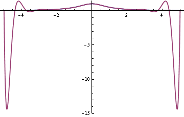
The fit is improving in the middle. In fact, the curves agree to within the thickness of the plot line from say −1 to 1. But the fit is so bad in the tails that the graph had to be cut off. Here’s another plot of f(x) and p16(x) on a different scale to show how far negative the polynomial dips.

graph of f(x) and p16(x) on different scale

The problem is the spacing of the nodes. Interpolation errors are bad for evenly spaced nodes.

Update: This post explains in a little more depth why this particular function has problems and gives another example where interpolation at evenly-spaced nodes behaves badly.

If we interpolate f(x) at different points, at the Chebyshev nodes, then the fit is good.

interpolating at Chebyshev nodes

The Chebyshev nodes on [−1, 1] are xi = cos( π i / n ). Here we multiplied these nodes by 5 to scale to the interval [−-5, 5].

If the function f(x) is absolutely continuous, as in our example, then the interpolating polynomials converge uniformly when you interpolate at Chebyshev nodes. However, ordinary continuity is not enough. Given any sequence of nodes, there exists a continuous function such that the polynomial interpolation error grows like log(n) as the number of nodes n increases.

Some numerical integration methods are based on interpolating polynomials: fit a polynomial to the integrand, then integrate the polynomial exactly to approximate the original integral. The examples above suggest that increasing the order of such integration methods might not improve accuracy and might even make things worse.

Related: Need help with interpolation?

Linear interpolator

I added a form to my website yesterday that does linear interpolation. If you enter (x1, y1) and (x2, y2), it will predict x3 given y3or vice versa by fitting a straight line to the first two points. It’s a simple calculation, but it comes up just often enough that it would be handy to have a page to do it.