Channel capacity of a telegraph

Claude Shannon’s famous paper A Mathematical Theory of Communication [1] includes an example saying that the channel capacity of a telegraph is log2 W where W is the largest real root of the determinant equation

\begin{vmatrix}-1 & W^{-2} + W^{-4} \\ W^{-3} + W^{-6} & W^{-2} + W^{-4} - 1 \end{vmatrix} = 0

Where in the world did that come from?

I’ll sketch where the equation above came from, but first let’s find W and log2 W.

Calculating channel capacity

If you take the determinant and multiply by W10 you get a 10th degree polynomial. A plot shows this polynomial has a root between 1.4 and 1.5.
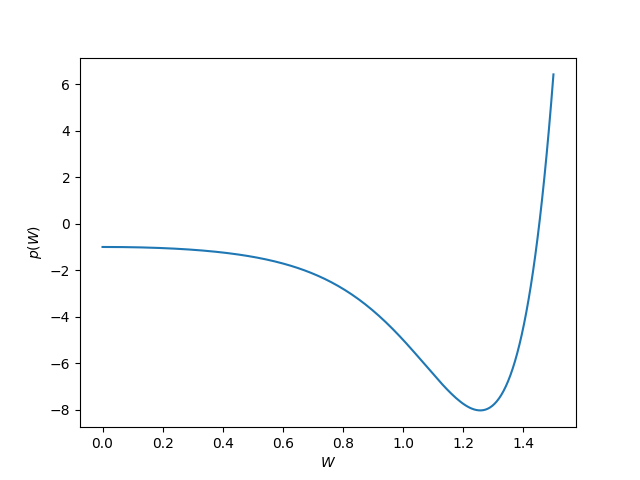
Applying the bisection method to that interval shows W = 1.4529 and so log2 W = 0.5389 which agrees with the value 0.539 that Shannon gives in his paper. This means that a telegraph can transmit a little more than one bit of information per unit time.

Interpretation

The result above means that a telegraph can transmit a little more than half a bit of information per unit time. But what is the unit of time implicit in Shannon’s example?

We think of Morse code as having two symbols—dot and dash—but in reality it has four symbols: dot, dash, intra-character space, and intra-word space. Shannon assumes that these four symbols take 2, 4, 3, and 6 units of time. Note that the time slice assigned to a dot or a dash includes enough silence at the end to distinguish dots and dashes.

Shannon does not assume that a telegraph is limited to send valid Morse code, only that it can transmit symbols of the four lengths discussed above, and that there are no consecutive spaces. He creates a finite automata model in which an intra-character space or an intra-word space can only transition to a dot or a dash.

Channel capacity

Shannon defines channel capacity in [1] as

C = \lim_{T\to\infty} \frac{\log_2 N(T)}{T}

where N(T) is the number of allowed signals of duration T. The hard part is calculating, or estimating, N(T). In the case of a telegraph, we can image calculating N(T) recursively via

N(t) = N(t - t_1) + N(t - t_2) + N(t - t_3) + N(t - t_4)

where the t‘s with subscripts are the times required to transmit each of the four possible symbols. The four terms on the right side consider the possibilities that the symbol transmitted immediately before time t is a dot, dash, intra-character space, or intra-word space.

The equation for N(t) is a finite difference equation, and so the asymptotic behavior of the solution is well known. Since we’re taking a limit as T goes to infinity, we only need to know the asymptotic behavior, so this works out well.

If you squint at the determinant at the top of the post, it looks sorta like an eigenvalue calculation, as hinted at by the −1 terms on the diagonal. And in fact that is what is going on. There’s an eigenvalue problem hidden in there that describes the asymptotic behavior of the difference equation.

Shannon’s theorem

Here is Theorem 1 from Shannon’s paper.

Let bij(s) be the duration of the sth symbol which is allowable in state i and leads to state j. The channel capacity C is equal to log2 W where W is the largest real root of the determinant equation

\left| \sum_s W^{-b_{ij}^{(s)}} - \delta_{ij} \right| = 0

where δij = 1 if i = j and is zero otherwise.

This theorem accounts for the determinant at the top of the post. It’s a 2 by 2 determinant because Shannon’s model of a telegraph is a finite automaton with two states, depending on whether the preceding symbol was or was not a space.

Related posts

[1] Claude Shannon. A Mathematical Theory of Communication. The Bell System Technical Journal, Vol. 27, pp. 379–423, July, October, 1948.

Edit distance

Newspaper editor

I was just talking to a colleague about edit distance because it came up in a project we’re working on.

Technically, we were discussing Levenshtein distance. It sounds more impressive to say Levenshtein distance, but it’s basically how much editing effort it would take to turn one block of text into another.

Edit distance is a fairly simple idea, and very useful. For example, the Morse code practice site LCWO [1] reports the Levenshtein distance between what you transcribe and the correct response. This better matches your intuitive idea of how well you did than some more direct ways of measuring accuracy. For example, transposing two characters is less of an error that typing two unrelated characters.

The LCWO site is unusual in that it explicitly reports Levenshtein distance. It’s far more common for the algorithm to be used behind the scenes and never mentioned by name.

Related posts

[1] Why “LCWO”? It stands for “learn CW online.” In the ham radio community, Morse code is usually called CW for historical reasons. CW stands for “continuous wave.” In principle you’re always transmitting at the same frequency, turning a carrier wave on and off, not modulating it. The details are a bit more interesting, as I write about here.

A surprising result about surprise index

Surprise index

Warren Weaver [1] introduced what he called the surprise index to quantify how surprising an event is. At first it might seem that the probability of an event is enough for this purpose: the lower the probability of an event, the more surprise when it occurs. But Weaver’s notion is more subtle than this.

Let X be a discrete random variable taking non-negative integer values such that

\text{Prob}(X = i) = p_i

Then the surprise index of the ith event is defined as

S_i = \frac{\sum_{j=0}^\infty p_j^2 }{p_i}

Note that if X takes on values 0, 1, 2, … N−1 all with equal probability 1/N, then Si = 1, independent of N. If N is very large, each outcome is rare but not surprising: because all events are equally rare, no specific event is surprising.

Now let X be the number of legs a human selected at random has. Then p2 ≈ 1, and so the numerator in the definition of Si is approximately 1 and S2 is approximately 1, but Si is large for any value of i ≠ 2.

The hard part of calculating the surprise index is computing the sum in the numerator. This is the same calculation that occurs in many contexts: Friedman’s index of coincidence, collision entropy in physics, Renyi entropy in information theory, etc.

Poisson surprise index

Weaver comments that he tried calculating his surprise index for Poisson and binomial random variables and had to admit defeat. As he colorfully says in a footnote:

I have spent a few hours trying to discover that someone else had summed these series and spent substantially more trying to do it myself; I can only report failure, and a conviction that it is a dreadfully sticky mess.

A few years later, however, R. M. Redheffer [2] was able to solve the Poisson case. His derivation is extremely terse. Redheffer starts with the generating function for the Poisson

e^{-\lambda} e^{\lambda x} = \sum p_mx^m

and then says

Let x = eiθ; then eiθ; multiply; integrate from 0 to 2π and simplify slightly to obtain

\sum p_m^2 = (e^{2\lambda}/\pi) \int_0^\pi e^{2\lambda \cos \theta}\, d\theta

The integral on the right is recognized as the zero-order Bessel function …

Redheffer then “recognizes” an expression involving a Bessel function. Redheffer acknowledges in a footnote at a colleague M. V. Cerrillo was responsible for recognizing the Bessel function.

It is surprising that the problem Weaver describes as a “dreadfully sticky mess” has a simple solution. It is also surprising that a Bessel function would pop up in this context. Bessel functions arise frequently in solving differential equations but not that often in probability and statistics.

Unpacking Redheffer’s derivation

When Redheffer says “Let x = eiθ; then eiθ; multiply; integrate from 0 to 2π” he means that we should evaluate both sides of the equation for the Poisson generating function equation at these two values of x, multiply the results, and average the both sides over the interval [0, 2π].

On the right hand side this means calculating

\frac{1}{2\pi} \int_0^{2\pi}\left(\sum_{m=0}^\infty p_m \exp(im\theta)\right) \left(\sum_{n=0}^\infty p_n \exp(-in\theta)\right)\, d\theta

This reduces to

\sum_{m=0}^\infty p_m^2

because

alt=

i.e. the integral evaluates to 1 when m = n but otherwise equals zero.

On the left hand side we have

\begin{align*} \frac{1}{2\pi} \int_0^{2\pi} \exp(-2\lambda) \exp(\lambda(e^{i\theta} + e^{-i\theta})) \, d\theta &= \frac{1}{2\pi} \int_0^{2\pi} \exp(-2\lambda) \exp(2 \cos \theta) \, d\theta \\ &= \frac{e^{-2\lambda}}{\pi} \int_0^{\pi} \exp(2 \cos \theta) \, d\theta \end{align*}

Cerrillo’s contribution was to recognize the integral as the Bessel function J0 evaluated at -2iλ or equivalently the modified Bessel function I0 evaluated at -2λ. This follows directly from equations 9.1.18 and 9.6.16 in Abramowitz and Stegun.

Putting it all together we have

\frac{\pi}{e^{2\lambda}}\sum_{m=0}^\infty p_m^2 = \int_0^{\pi} \exp(2 \cos \theta) \, d\theta = J_0(-2i\lambda ) = I_0(-2\lambda )

Using the asymptotic properties of I0 Redheffer notes that for large values of λ,

\sum_{m=0}^\infty p_m^2 \sim \frac{1}{2\sqrt{\pi\lambda}}

[1] Warren Weaver, “Probability, rarity, interest, and surprise,” The Scientific Monthly, Vol 67 (1948), p. 390.

[2] R. M. Redheffer. A Note on the Surprise Index. The Annals of Mathematical Statistics, Mar., 1951, Vol. 22, No. 1 pp. 128ndash;130.

When is less data less private?

If I give you a database, I give you every row in the database. So if you delete some rows from the database, you have less information, not more, right?

This seems very simple, and it mostly is, but there are a couple subtleties.

A common measure in data privacy is k-anonymity. The idea is that if at least k individuals in a data set share some set of data values, and k is large enough, then the privacy of those individuals is protected.

Now suppose you randomly select a single record from a database that was deemed deidentified because it satisfied k-anonymity with k = 10. Now your new dataset, consisting of only one record, is k-anonymous with k = 1: every record is unique because there’s only one record. But how is this person’s data any less private that it was before?

Note that I said above that you selected a record at random. If you selected the row using information that you know but which isn’t in the database, you might have implicitly added information. But if you select a subset of data, using only information explicit in that data, you haven’t added information.

Here’s where k-anonymity breaks down. The important measure is k-anonymity in the general population, not k-anonymity in a data set, unless you know that someone is in the data set.

If you find someone named John Cook in a data set, you probably haven’t found my information, even if there is only one person by that name in the data set. My name may or may not be common in that particular data set, but my name is common in general.

The number of times a combination of data fields gives a lower bound on how often the combination appears in general, so k-anonymity in a data set is a good sign for privacy, but the lack of k-anonymity is not necessarily a bad sign. The latter could just be an artifact of having a small data set.

Related posts

KL divergence from normal to normal

The previous post looked at the best approximation to a normal density by normal density with a different mean. Dan Piponi suggested in the comments that it would be good to look at the Kullback-Leibler (KL) divergence.

The previous post looked at the difference from between two densities from an analytic perspective, solving the problem that an analyst would find natural. This post takes an information theoretic perspective. Just is p-norms are natural in analysis, KL divergence is natural in information theory.

The Kullback-Leibler divergence between two random variables X and Y is defined as

KL(X || Y) = -\int f_X(x) \log \frac{f_Y(x)}{f_X(x)} \, dx

There are many ways to interpret KL(X || Y), such as the average surprise in seeing Y when you expected X.

Unlike the p-norm distance, the KL divergence between two normal random variables can be computed in closed form.

Let X be a normal random variable with mean μX and variance σ²X and Y a normal random variable with mean μY and variance σ²Y. Then

KL(X || Y) = \log\frac{\sigma_Y}{\sigma_X} + \frac{\sigma_X^2 + (\mu_X - \mu_Y)^2}{2\sigma_Y^2} - \frac{1}{2}

If μX = 0 and σX = 1, then for fixed μY the value of σ²Y that minimizes KL(X || Y) is

\sigma_Y^2 = 1 + \mu_Y^2

KL divergence is not symmetric, hence we say divergence rather than distance. More on that here. If we want to solve the opposite problem, minimizing KL(X || Y), the optimal value of σ²Y is simply 1.

Differential entropy and privacy

Differential entropy is the continuous analog of Shannon entropy. Given a random variable X with density function fX, the differential entropy of X, denoted h(X), is defined as

h(X) = -\int f_X(x) \log_2 f_X(x)\, dx

where the integration is over the support of fX. You may see differential entropy defined using logarithm to a different base, which changes h(X) by a constant amount.

In [1] the authors defined the privacy of a random variable X, denoted Π(X), as 2 raised to the power h(X).

\Pi(X) = 2^{h(X)}

This post will only look at “privacy” as defined above. Obviously the authors chose the name because of its application to privacy in the colloquial sense, but here we will just look at the mathematics.

Location and scale

It follows directly from the definitions above that location parameters do not effect privacy, and scale parameters change privacy linearly. That is, for σ > 0,

\Pi(\sigma X + \mu) = \sigma \,\Pi(X)

If we divide by standard deviation before (or after) computing privacy then we have a dimensionless quantity. Otherwise there’s more privacy is measuring a quantity in centimeters than in measuring it in inches, which is odd since both contain the same information.

Examples

If X is uniformly distributed on an interval of length a, then h(X) = log2 a and Π(X) = a.

The privacy of a standard normal random variable Z is √(2πe) and so the privacy of a normal random variable with mean μ and variance σ² is σ√(2πe).

The privacy of a standard exponential random variable is 1, so the privacy of an exponential with rate λ is 1/λ.

Bounds

A well-known theorem says that for given variance, differential entropy is maximized by a normal random variable. This means that the privacy of a random variable with variance σ² is bounded above by σ√(2πe).

The privacy of a Cauchy random variable with scale σ is 4πσ, which is greater than σ√(2πe). This is does not contradict the statement above because the scaling parameter of a Cauchy random variable is not its standard deviation. A Cauchy random variable does not have and standard deviation.

Related posts

[1] Agrawal D., Aggrawal C. C. On the Design and Quantification of Privacy-Preserving Data Mining Algorithms, ACM PODS Conference, 2002. (Yes, the first author’s name contains one g and the second author’s name contains two.)

Identifiers depend on context

Can you tell who someone is from their telephone number? That’s kinda the point of telephone numbers, to let you contact someone. And indeed telephone number is one the 18 identifiers under HIPAA Safe Harbor.

But whether any piece of information allows you to identify someone depends on context. If you don’t have access to a phone, or a phone book, or any electronic counterpart of a phone book, then a phone number doesn’t allow you to identify anyone. But once you can call a phone number or enter it into a search engine, then the phone number is identifiable. Maybe.

What if the number belongs to a burner phone? Then it would be harder to learn the identity of the person who owns the number, but not impossible. Maybe you couldn’t learn anything about the owner, but law enforcement officials could. Again identifiability depends on context.

An obvious identifier like a phone number might not be an identifier in some special circumstance. And an apparently useless bit of information might reveal someone’s identity in another circumstance.

HIPAA’s Safe Harbor Rule tries to say apart from context what kinds of data are identifiable. But if you read the Safe Harbor Rule carefully you’ll notice it isn’t so context-free as it seems. The last item in the list of 18 items to remove is “any other unique identifying number, characteristic, or code.” What might be an identifying characteristic? That depends on context.

Logarithms yearning to be free

I got an evaluation copy of The Best Writing on Mathematics 2021 yesterday. One article jumped out as I was skimming the table of contents: A Zeroth Power Is Often a Logarithm Yearning to Be Free by Sanjoy Mahajan. Great title.

There are quite a few theorems involving powers that have an exceptional case that involves a logarithm. The author opens with the example of finding the antiderivative of xn. When n ≠ −1 the antiderivative is another power function, but when n = −1 it’s a logarithm.

Another example that the author mentions is that the limit of power means as the power goes to 0 is the geometric mean. i.e. the exponential of the mean of the logarithms of the arguments.

I tried to think of other examples where this pattern pops up, and I thought of a couple related to entropy.

q-logarithm entropy

The definition of q-logarithm entropy takes Mahajan’s idea and runs it backward, turning a logarithm into a power. As I wrote about here,

The natural logarithm is given by

\ln(x) = \int_1^x t^{-1}\,dt

and we can generalize this to the q-logarithm by defining

\ln_q(x) = \int_1^x t^{-q}\,dt

And so ln1 = ln.

Then q-logarithm entropy is just Shannon entropy with natural logarithm replaced by q-logarithm.

Rényi entropy

Quoting from this post,

If a discrete random variable X has n possible values, where the ith outcome has probability pi, then the Rényi entropy of order α is defined to be

H_\alpha(X) = \frac{1}{1 - \alpha} \log_2 \left(\sum_{i=1}^n p_i^\alpha \right)

for 0 ≤ α ≤ ∞. In the case α = 1 or ∞ this expression means the limit as α approaches 1 or ∞ respectively.

When α = 1 we get the more familiar Shannon entropy:

H_1(X) = \lim_{\alpha\to1} H_\alpha(X) = - \left(\sum_{i=1}^n p_i \log_2 p_i \right)

In this case there’s already a logarithm in the definition, but it moves inside the parentheses in the limit.

And if you rewrite

pα

as

p pα−1

then as the exponent in pα−1 goes to zero, we have a logarithm yearning to be free.

Related

Information in a discretized normal

Here’s a problem that came up in my work today.

Suppose you have a normal random variable X and you observe X in n discrete bins. The first bin is the left α tail, the last bin is the right α tail, and the range between the two tails is divided evenly into n-2 intervals. How many bits of information are in such an observation?

For example, assume adult male heights are normally distributed with mean 70 inches and standard deviation 3 inches. How much information is there in an observation of height, rounded down to the nearest inch, if we put all heights less than 64 inches in a bin and all heights greater than or equal to 76 inches in a bin?

Here α = 0.025 because that’s the probability that a normal random variable is more than 2 standard deviations below its mean or more than 2 standard deviations above its mean.

We have n = 15 because we have intervals (-∞, 64), [64, 65), [65, 66), … [75, 76), and [76, ∞).

We know that with n bins we have at most log2n bits of information. That would correspond to n bins of equal probability. In other words, we’d get the maximum information if we spaced our bins evenly in terms of percentiles rather in terms of inches.

So how does the information content vary as a function of the number of bins, and how close is it to the maximum information for n bins?

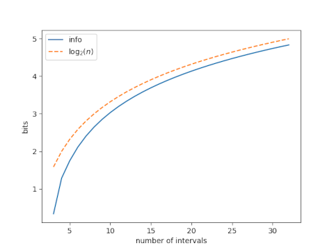
Here’s a plot, with α = 0.025.

The suboptimality of our bins, i.e. the difference between log2n and the information we get from n bins, drops quickly at first as n increases, then appears to plateau.

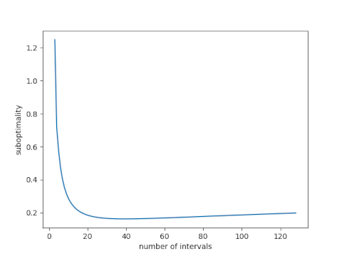
Next lets look at just the suboptimality, and increase our range of n.

This shows that the suboptimality does not approach an asymptote but instead starts to increase. The minimum at n = 36 is 0.16 bits.

Information loss and entropy

John Baez, Tobias Fritz, and Tom Leinster wrote a nice paper [1] that shows Shannon entropy is the only measure of information loss that acts as you’d expect, assuming of course you have the right expectations. See their paper for all the heavy lifting. All I offer here is an informal rewording of the hypotheses.

The authors say that

We show that Shannon entropy gives the only concept of information loss that is functorial, convex-linear and continuous.

You could reword this by saying

Shannon entropy is the only measure of information loss that composes well, mixes well, and is robust.

Saying that a measure of information loss composes well means that the information lost by doing two processes f and then g is the sum of the information lost by doing f and the information lost by doing g. This is what the authors describe as functorial.

When I refer to something mixing well, I have in mind mixtures in the sense of probability. A mixture is a random choice of random variables, such as flipping a coin to decide which of two dice to roll.

Going back to our two processes f and g, if we choose to do f with probability p and to do g with probability (1 – p) then the information loss from this mixture process should be p times the information loss from f plus (1-p) times the information lost from g. Instead of saying this mixes well, you could say it behaves as expected, where “as expected” is a pun on expected value. The authors describe this as convex-linear because the expected information loss is a convex combination of the two possible losses.

Robustness is a more colloquial term for continuity. Something is robust if small changes in inputs should lead to small changes in outputs. If you make this statement rigorous, you end up with the definition of continuity. If we change a process f a little then we should change our measure of information loss a little.

More on information theory

[1] A characterization of entropy in terms of information loss. On arXiv.