A convergence problem going around Twitter

Ten days ago, Fermat’s library posted a tweet saying that it is unknown whether the sum

\sum_{n=1}^\infty \frac{1}{n^3 \sin(n)^2}

converges or diverges, stirring up a lot of discussion. Sam Walters has been part of this discussion and pointed to a paper that says this is known as the Flint Hills series.

My first thought was to replace the sine term with a random variable and see what happens, because the values of n mod 2π act a lot like a random sequence. To be precise, the series is ergodic.

If X is a uniform random variable on the interval [0, 2π], then the random variable Y = 1/sin(X)² is fat tailed, so fat that it has no finite expected value. If Y had a finite expected value E[Y], then one might expect the Flint Hills sum to be roughly E[Y] ζ(3), i.e. the Flint Hills sum with the sine terms replaced by E[Y]. But since E[Y] diverges, this suggests that the Flint Hills series diverges.

Of course this doesn’t settle the question because the values of n mod 2π are not actually random. They simply act as if they were random in some contexts. For example, if you wanted to use them as if they were random values in order to do Monte Carlo integration, they would work just fine.

The question is whether the values act sufficiently like random values in the context of the Flint Hills problem. This is not clear, and is a problem in number theory rather than in probability. (Though number theory and probability are surprisingly interconnected.)

Sam Walters suggested considering a variation on the Flint Hills problem where we replace sin(n) with sin(2πθn) for some constant θ, the original problem corresponding to θ = 1/2π. I suspect the series diverges for some (almost all?) values of θ. That is, unless you pick θ very carefully, number theory won’t rescue the series from divergence.

Related posts

The other butterfly effect

monarch butterfly

The original butterfly effect

The butterfly effect is the semi-serious claim that a butterfly flapping its wings can cause a tornado half way around the world. It’s a poetic way of saying that some systems show sensitive dependence on initial conditions, that the slightest change now can make an enormous difference later. Often this comes up in the context of nonlinear, chaotic systems but it isn’t limited to that. I give an example here of a linear differential equation whose solutions start out the essentially the same but eventually diverge completely.

Once you think about these things for a while, you start to see nonlinearity and potential butterfly effects everywhere. There are tipping points everywhere waiting to be tipped!

The other butterfly effect

But a butterfly flapping its wings usually has no effect, even in sensitive or chaotic systems. You might even say especially in sensitive or chaotic systems.

Sensitive systems are not always and everywhere sensitive to everything. They are sensitive in particular ways under particular circumstances, and can otherwise be quite resistant to influence. Not only may a system be insensitive to butterflies, it may even be relatively insensitive to raging bulls. The raging bull may have little more long-term effect than a butterfly. This is what I’m calling the other butterfly effect.

Steering complex systems

In some ways chaotic systems are less sensitive to change than other systems. And this can be a good thing. Resistance to control also means resistance to unwanted tampering. Chaotic or stochastic systems can have a sort of self-healing property. They are more stable than more orderly systems, though in a different way.

The lesson that many people draw from their first exposure to complex systems is that there are high leverage points, if only you can find them and manipulate them. They want to insert a butterfly to at just the right time and place to bring about a desired outcome. Instead, we should humbly evaluate to what extent it is possible to steer complex systems at all. We should evaluate what aspects can be steered and how well they can be steered. The most effective intervention may not come from tweaking the inputs but from changing the structure of the system.

More dynamical systems posts

A uniformly distributed sequence

If you take the fractional parts of the set of numbers {n cos nx :  integer n > 0} the result is uniformly distributed for almost all x. That is, in the limit, the number of times the sequence visits a subinterval of [0, 1] is proportional to the length of the interval. (Clearly it’s not true for all x: take x = 0, for instance. Or any rational number times π.)

The proof requires some delicate work with Fourier analysis that I’ll not repeat here. If you’re interested in the proof, see Theorem 4.4 of Uniform Distribution of Sequences.

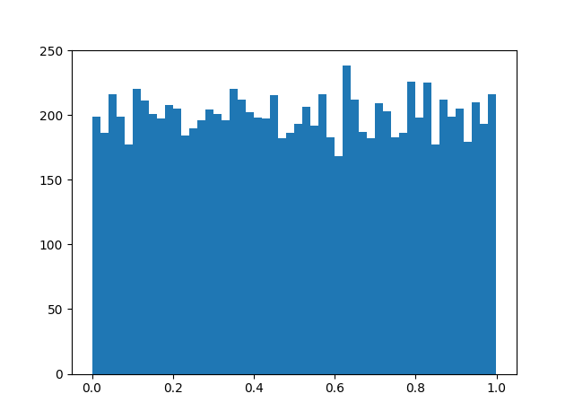
This is a surprising result: why should such a strange sequence be uniformly distributed? Let’s look at a histogram to see whether the theorem is plausible.


Histogram for an = n

OK. Looks plausible.

But there’s a generalization that’s even more surprising. Let an be any increasing sequence of integers. Then the fractional parts of an cos anx are uniformly distributed for almost all x.

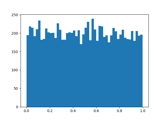
Any increasing sequence of integers? Like the prime numbers, for example? Apparently so. The result produces a very similar histogram.

Histogram for an = n

But this can’t hold for just any sequence. Surely you could pick an integer sequence to thwart the theorem. Pick an x, then let an be the subset of the integers for which n cos nx < 0.5. Then an cos anx isn’t uniformly distributed because it never visits the right half the unit interval!

Where’s the contradiction? The theorem doesn’t start by saying “For almost all x ….” It starts by saying “For any increasing sequence an ….” That is, you don’t get to pick x first. You pick the sequence first, then you get a statement that is true for almost all x. The theorem is true for every increasing sequence of integers, but the exceptional set of x‘s may be different for each integer sequence.

Chaos and the beta distribution

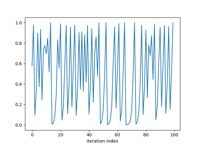
Iteration of the quadratic function f(x) = 4x(1-x) is a famous example in chaos theory. Here’s what the first few iterations look like, starting with 1/√3. (There’s nothing special about that starting point; any point that doesn’t iterate to exactly zero will do.)

quadratic iterator first 100 values

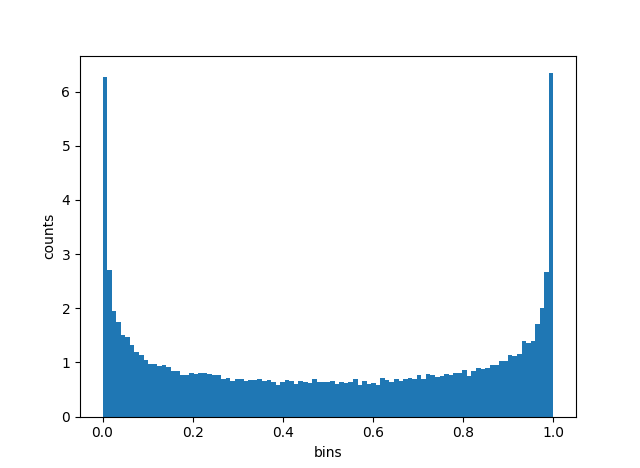
The values appear to bounce all over the place. Let’s look at a histogram of the sequence.

histogram

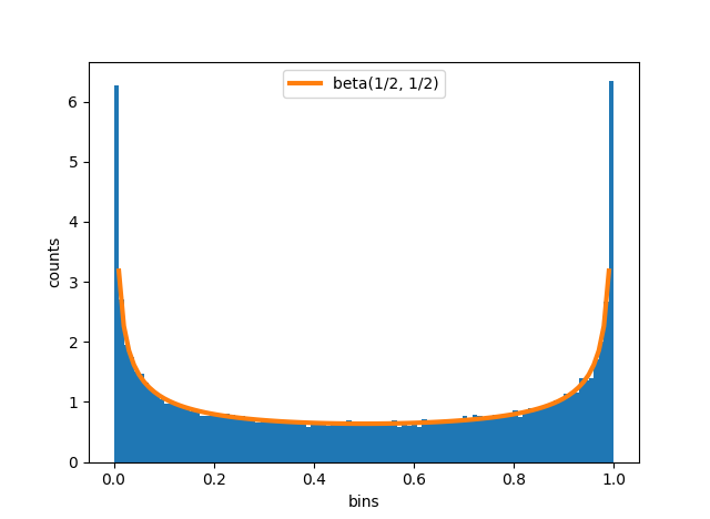
Indeed the points do bounce all over the unit interval, though they more often bounce near one of the ends.

Does that distribution look familiar? You might recognize it from Bayesian statistics. It’s a beta distribution. It’s symmetric, so the two beta distribution parameters are equal. There’s a vertical asymptote on each end, so the parameters are less than 1. In fact, it’s a beta(1/2, 1/2) distribution. It comes up, for example, as the Jeffreys prior for Bernoulli trials.

The graph below adds the beta(1/2, 1/2) density to the histogram to show how well it fits.

histogram with beta density

We have to be careful in describing the relation between the iterations and the beta distribution. The iterates are ergodic, not random. The sequence of points does not simulate independent draws from any distribution: points near 0.5 are always sent to points near 1, points near 1 are always sent to points near 0, etc. But in aggregate, the points do fill out the unit interval like samples from a beta distribution. In the limit, the proportion of points in a region equals the probability of that region under a beta(1/2, 1/2) distribution.

Here’s the Python code that produced the graphs above.

import numpy as np
from scipy.stats import beta
import matplotlib.pyplot as plt

def quadratic(x):
    return 4*x*(1-x)

N = 100000
x = np.empty(N)

# arbitrary irrational starting point
x[0] = 1/np.sqrt(3) 
for i in range(1, N):
    x[i] = quadratic( x[i-1] )

plt.plot(x[0:100])
plt.xlabel("iteration index")
plt.show()

t = np.linspace(0, 1, 100)
plt.hist(x, bins=t, normed=True)
plt.xlabel("bins")
plt.ylabel("counts")

plt.plot(t, beta(0.5,0.5).pdf(t), linewidth=3)
plt.legend(["beta(1/2, 1/2)"])
plt.show()

More ergodic theory posts

Polynomials evaluated at integers

Let p(x) = a0 + a1x + a2x2 + … + anxn and suppose at least one of the coefficients ai is irrational for some i ≥ 1. Then a theorem by Weyl says that the fractional parts of p(n) are equidistributed as n varies over the integers. That is, the proportion of values that land in some interval is equal to the length of that interval.

Clearly it’s necessary that one of the coefficients be irrational. What may be surprising is that it is sufficient.

If the coefficients are all rational with common denominator N, then the sequence would only contain multiples of 1/N. The interval [1/3N, 2/3N], for example, would never get a sample. If a0 were irrational but the rest of the coefficients were rational, we’d have the same situation, simply shifted by a0.

This is a theorem about what happens in the limit, but we can look at what happens for some large but finite set of terms. And we can use a χ2 test to see how evenly our sequence is compared to what one would expect from a random sequence.

In the Python code below, we use the polynomial p(x) = √2 x² + πx + 1 and evaluate p at 0, 1, 2, …, 99,999. We then count how many fall in the bins [0, 0.01), [0.01, 0.02), … [0.99, 1] and compute a chi-square statistic on the counts.

from math import pi, sqrt, floor

def p(x):
    return 1 + pi*x + sqrt(2)*x*x

def chisq_stat(O, E):
    return sum( (o - e)**2/e for (o, e) in zip(O, E) )

def frac(x):
    return x - floor(x)

N = 100000
data = [frac(p(n)) for n in range(N)]

count = [0]*100
for d in data:
    count[ int(floor(100*d)) ] += 1

expected = [N/100]*100

print(chisq_stat(count, expected))

We get a chi-square statistic of 95.4. Since we have 100 bins, there are 99 degrees of freedom, and we should compare our statistic to a chi-square distribution with 99 degrees of freedom. Such a distribution has mean 99 and standard deviation √(99*2) = 14.07, so a value of 95.4 is completely unremarkable.

If we had gotten a very large chi-square statistic, say 200, we’d have reason to suspect something was wrong. Maybe a misunderstanding on our part or a bug in our software. Or maybe the sequence was not as uniformly distributed as we expected.

If we had gotten a very small chi-square statistic, say 10, then again maybe we misunderstood something, or maybe our sequence is remarkably evenly distributed, more evenly than one would expect from a random sequence.

Related math posts

Leading digits of powers of 2

The first digit of a power of 2 is a 1 more often than any other digit. Powers of 2 begin with 1 about 30% of the time. This is because powers of 2 follow Benford’s law. We’ll prove this below.

When is the first digit of 2n equal to k? When 2n is between k × 10p and (k + 1) × 10p for some positive integer p. By taking logarithms base 10 we find that this is equivalent to the fractional part of n log102 being between log10 k and log10 (k + 1).

The map

x ↦ ( x + log10 2 ) mod 1

is ergodic. I wrote about irrational rotations a few weeks ago, and this is essentially the same thing. You could scale x by 2π and think of it as rotations on a circle instead of arithmetic mod 1 on an interval. The important thing is that log10 2 is irrational.

Repeatedly multiplying by 2 is corresponds to adding log10 2 on the log scale. So powers of two correspond to iterates of the map above, starting with x = 0. Birkhoff’s Ergodic Theorem tells us that the number of times iterates of this map fall in the interval [ab] equals b – a. So for k = 1, 2, 3, … 9, the proportion of powers of 2 start with k is equal to  log10 (k + 1) –  log10 (k) =  log10 ((k + 1) / k).

This is Benford’s law. In particular, the proportion of powers of 2 that begin with 1 is equal to  log10 (2) = 0.301.

Note that the only thing special about 2 is that log10 2 is irrational. Powers of 3 follow Benford’s law as well because log10 3 is also irrational. For what values of b do powers of b not follow Benford’s law? Those with log10 b rational, i.e. powers of 10. Obviously powers of 10 don’t follow Benford’s law because their first digit is always 1!

[Interpret the “!” above as factorial or exclamation as you wish.]

Let’s look at powers of 2 empirically to see Benford’s law in practice. Here’s a simple Python program to look at first digits of powers of 2.

count = [0]*10
N = 10000

def first_digit(n):
    return int(str(n)[0])

for i in range(N):
    n = first_digit( 2**i )
    count[n] += 1

print(count)

Unfortunately this only works for moderate values of N. It ran in under a second with N set to 10,000 but for larger values of N it rapidly becomes impractical.

Here’s a much more efficient version that ran in about 2 seconds with N = 1,000,000.

from math import log10
N = 1000000
count = [0]*10

def first_digit_2_exp_e(e):
    r = (log10(2.0)*e) % 1
    for i in range(2, 11):
        if r < log10(i):
            return i-1
for i in range(N):
    n = first_digit_2_exp_e( i )
    count[n] += 1

print(count)

You could make it more efficient by caching the values of log10 rather than recomputing them. This brought the run time down to about 1.4 seconds. That’s a nice improvement, but nothing like the orders of magnitude improvement from changing algorithms.

Here are the results comparing the actual counts to the predictions of Benford’s law (rounded to the nearest integer).

|---------------+--------+-----------|
| Leading digit | Actual | Predicted |
|---------------+--------+-----------|
|             1 | 301030 |    301030 |
|             2 | 176093 |    176091 |
|             3 | 124937 |    124939 |
|             4 |  96911 |     96910 |
|             5 |  79182 |     79181 |
|             6 |  66947 |     66948 |
|             7 |  57990 |     57992 |
|             8 |  51154 |     51153 |
|             9 |  45756 |     45757 |
|---------------+--------+-----------|

The agreement is almost too good to believe, never off by more than 2.

Are the results correct? The inefficient version relied on integer arithmetic and so would be exact. The efficient version relies on floating point and so it’s conceivable that limits of precision caused a leading digit to be calculated incorrectly, but I doubt that happened. Floating point is precise to about 15 significant figures. We start with log10(2), multiply it by numbers up to 1,000,000 and take the fractional part. The result is good to around 9 significant figures, enough to correctly calculate which log digits the result falls between.

Update: See Andrew Dalke’s Python script in the comments. He shows a way to efficiently use integer arithmetic.

Related: Benford’s law posts sorted by application area

Fractional parts, invariant measures, and simulation

A function f: XX is measure-preserving if for each iteration of f sends the same amount of stuff into a given set. To be more precise, given a measure μ and any μ-measurable set E with μ(E) > 0, we have

\mu( E ) = \mu( f^{-1}(E) )

You can read the right side of the equation above as “the measure of the set of points that f maps into E.” You can apply this condition repeatedly to see that the measure of the set of points mapped into E after n iterations is still just the measure of E.

If X is a probability space, i.e. μ( ) = 1, then you could interpret the definition of measure-preserving to mean that the probability that a point ends up in E after n iterations is independent of n. We’ll illustrate this below with a simulation.

Let X be the half-open unit interval (0, 1] and let f be the Gauss map, i.e.

f(x) = \frac{1}{x} - \left\lfloor \frac{1}{x}\right\rfloor

where [z] is the integer part of z. The function f is measure-preserving, though not for the usual Lebesgue measure. Instead it preserves the following measure:

\mu(E) = \frac{1}{\log 2} \int_E \frac{1}{1+x} \, dx

Let’s take as our set E an interval [a, b] and test via simulation whether the probability of landing in E after n iterations really is just the measure of E, independent of n.

We can’t just generate points uniformly in the interval (0, 1]. We have to generate the points so that the probability of a point coming from a set E is μ(E). That means the PDF of the distribution must be p(x) = 1 / (log(2) (1 + x)). We use the inverse-CDF method to generate points with this density in the Python code below.

from math import log, floor
from random import random

def gauss_map(x):
    y = 1.0/x
    return y - floor(y)

# iterate gauss map n times
def iterated_gauss_map(x, n):
    while n > 0:
        x = gauss_map(x)
        n = n - 1
    return x      

# measure mu( [a,b] )
def mu(a, b):
    return (log(1.0+b) - log(1.0+a))/log(2.0)

# Generate samples with Prob(x in E) = mu( E )
def sample():
    u = random()
    return 2.0**u - 1.0

def simulate(num_points, num_iterations, a, b):
    count = 0
    for _ in range(num_points):
        x = sample()
        y = iterated_gauss_map(x, num_iterations)
        if a < y < b:
            count += 1
    return count / num_points

# Change these parameters however you like
a, b = 0.1, 0.25
N = 1000000

exact = mu(a, b)
print("Exact probability:", exact)
print("Simulated probability after n iterations")
for n in range(1, 10):
    simulated = simulate(N, n, a, b)
    print("n =", n, ":", simulated)

Here’s the output I got:

Exact probability: 0.18442457113742736
Simulated probability after n iterations
n = 1 : 0.184329
n = 2 : 0.183969
n = 3 : 0.184233
n = 4 : 0.184322
n = 5 : 0.184439
n = 6 : 0.184059
n = 7 : 0.184602
n = 8 : 0.183877
n = 9 : 0.184834

With 1,000,000 samples, we expect the results to be the same to about 3 decimal places, which is what we see above.

Related post: Irrational rotations are ergodic.

(A transformation f  is ergodic if it is measure preserving and the only sets E with  f –1(E)  = E are those with measure 0 or full measure. Rational rotations are measure-preserving but not ergodic. The Gauss map above is ergodic.)

Irrational rotations are ergodic

In a blog post yesterday, I mentioned that the golden angle is an irrational portion of a circle, and so a sequence of rotations by the golden angle will not repeat itself. We can say more: rotations by an irrational portion of a circle are ergodic. Roughly speaking, this means that not only does the sequence not repeat itself, the sequence “mixes well” in a technical sense.

Ergodic functions have the property that “the time average equals the space average.” We’ll unpack what that means and illustrate it by simulation.

Suppose we pick a starting point x on the circle then repeatedly rotate it by a golden angle. Take an integrable function f on the circle and form the average of its values at the sequence of rotations. This is the time average. The space average is the integral of f over the circle, divided by the circumference of the circle. The ergodic theorem says that the time average equals the space average, except possibly for a setting of starting values of measure zero.

More generally, let X be a measure space (like the unit circle) with measure μ let T be an ergodic transformation (like rotating by a golden angle), Then for almost all starting values x we have the following:

\lim_{n\to \infty} \frac{1}{n} \sum_{k=0}^{n-1} f(T^k x) = \frac{1}{\mu(X)} \int_X f\, d\mu

Let’s do a simulation to see this in practice by running the following Python script.

        from scipy import pi, cos
        from scipy.constants import golden
        from scipy.integrate import quad
        
        golden_angle = 2*pi*golden**-2
        
        def T(x):
            return (x + golden_angle) % (2*pi)
        
        def time_average(x, f, T, n):
            s = 0
            for k in range(n):
                s += f(x)
                x = T(x)
            return s/n
        
        def space_average(f):
            integral = quad(f, 0, 2*pi)[0]
            return integral / (2*pi)
        
        f = lambda x: cos(x)**2
        N = 1000000
        
        print( time_average(0, f, T, N) )
        print( space_average(f) )

In this case we get 0.49999996 for the time average, and 0.5 for the space average. They’re not the same, but we only used a finite value of n; we didn’t take a limit. We should expect the two values to be close because n is large, but we shouldn’t expect them to be equal.

Update: The code and results were updated to fix a bug pointed out in the comments below.  I had written ... % 2*pi when I should have written ... % (2*pi). I assumed the modulo operator was lower precedence than multiplication, but it’s not. It was a coincidence that the buggy code was fairly accurate.

A friend of mine, a programmer with decades of experience, recently made a similar error. He’s a Clojure fan but was writing in C or some similar language. He rightfully pointed out that this kind of error simply cannot happen in Clojure. Lisps, including Clojure, don’t have operator precedence because they don’t have operators. They only have functions, and the order in which functions are called is made explicit with parentheses. The Python code x % 2*pi corresponds to (* (mod x 2) pi) in Clojure, and the Python code x % (2*pi) corresponds to (mod x (* 2 pi)).

Related: Origin of the word “ergodic”

Ergodic

Roughly speaking, an ergodic system is one that mixes well. You get the same result whether you average its values over time or over space.

This morning I ran across the etymology of the word:

In the late 1800s, the physicist Ludwig Boltzmann needed a word to express the idea that if you took an isolated system at constant energy and let it run, any one trajectory, continued long enough, would be representative of the system as a whole. Being a highly-educated nineteenth century German-speaker, Boltzmann knew far too much ancient Greek, so he called this the “ergodic property”, from ergon “energy, work” and hodos “way, path.” The name stuck.

Found here, footnote on page 479.

More posts on ergodic systems: