Complex golden convergence

Posted on 23 February 2025 by John

The previous post looked at how iterations of

$x \mapsto \sqrt{1 + x}$

converge to the golden ratio φ. That post said we could start at any positive x. We could even start at any x > −¾ because that would be enough for the derivative of √(1 + x) to be less than 1, which means the iteration will be a contraction.

We can’t start at any x less than −1 because then our square root would be undefined, assuming we’re working over real numbers. But what if we move over to the complex plane?

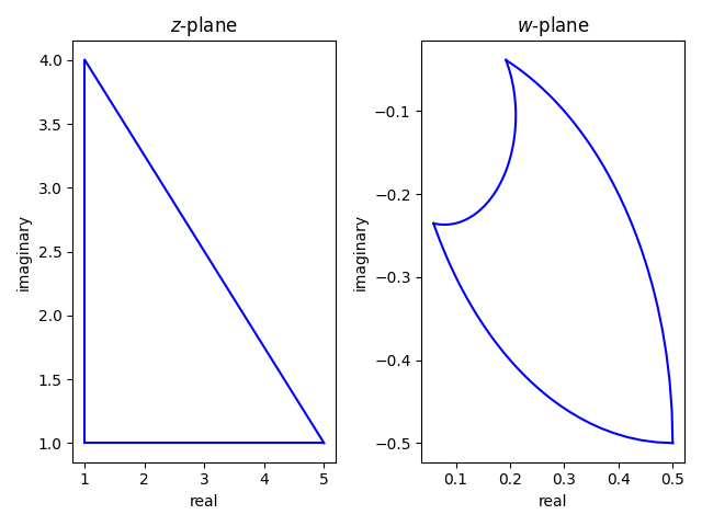
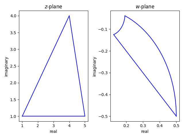
If f is a real-valued function of a real variable and|f ′(x)| is bounded by a constant less than 1 on an interval, then f is a contraction on that interval. Is the analogous statement true for a complex-valued function of a complex variable? Indeed it is.

If we start at a distance at least ¼ away from −1 then we have a contraction and the iteration converges to φ. If we start closer than that to −1, then the first step of the iteration will throw us further out to where we then converge.

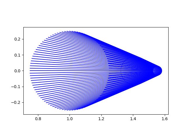
To visualize the convergence, let’s look at starting at a circle of points in a circle of radius 10 around φ and tracing the path of each iteration.

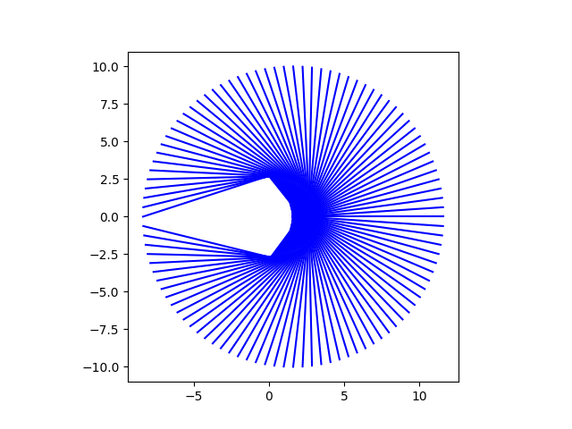
For most of the starting points, the iterations converge almost straight toward φ, but points near the negative real axis take a more angular path. The gap in the plot is an artifact of iterations avoiding the disk of radius ¼ around −1. Let’s see what happens when we start on the boundary of this disk.

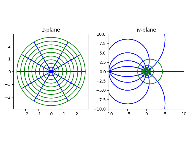
Next, instead of connecting each point to its next iteration, let’s plot the starting circle, then the image of that circle, and the image of that circle, etc.

The boundary of the disk, the blue circle, is mapped to the orange half-circle, which is then mapped to the green stretched half circle, etc.

1 + 2 + 3 + … = −1/12

Posted on 13 February 2025 by John

The other day MathMatize posted

roses are red
books go on a shelf
1+2+3+4+ …

with a photo of Ramanujan on X.

This was an allusion to the bizarre equation

1 + 2 + 3 + … = − 1/12.

This comes up often enough that I wanted to write a post that I could share a link to next time I see it.

The equation is nonsense if interpreted in the usual way. The sum on the left diverges. You could say the sum is ∞ if by that you mean you can make the sum as large as you like by taking the partial sum out far enough.

Here’s how the equation is mean to be interpreted. The Riemann zeta function is defined as

$\zeta(s) = \sum_{n=1}^\infty \frac{1}{n^s}$

for complex numbers s with positive real part, and defined for the rest of the complex plane by analytic continuation. The qualifiers matter. The infinite sum above does not define the zeta function for all numbers; it defines ζ(s) for numbers with real part greater than 1. The sum is valid for numbers like 7, or 42 −476i, or √2 + πi, but not for −1.

If the sum did define ζ(−1) then the sum would be 1 + 2 + 3 + …, but it doesn’t.

However, ζ(−1) is defined, and it equals −1/12.

What does it mean to define a function by analytic continuation? There is a theorem that essentially says there is only one way to extend an analytic function. It is possible to construct an analytic function that has the same values as ζ(s) when Re(s) > 1, where that function is defined for all s ≠ 1.

We could give that function a new name, say f(s). That is the function whose value at −1 equals − 1/12. But since there is only one possible analytic function f that overlaps with ζ(s) we go ahead and use the notation ζ(s) for this extended function.

To put it another way, the function ζ(s) is valid for all s ≠ 1, but the series representation for ζ(s) is not valid unless Re(s) > 1. There are other representations for ζ(s) for other regions of the complex plane, including for s = −1, and that’s what lets us compute ζ(−1) to find out that it equals −1/12.

So the rigorous but less sensational way to interpret the equation is to say

1^−s + 2^−s + 3^−s + …

is a whimsical way of referring to the function defined by the series, when the series converges, and defined by its analytic continuation otherwise. So in addition to saying

1 + 2 + 3 + … = − 1/12

we could also say

1² + 2² + 3² + … = 0

and

1³ + 2³ + 3³ + … = 1/120.

You can make up your own equation for any value of s for which you can calculate ζ(s).

Duplicating Hankel plot from A&S

Posted on 22 January 2025 by John

Abramowitz and Stegun has quite a few intriguing plots. The post will focus on the follow plot, Figure 9.4, available here.

A&S figure 9.4

We will explain what the plot is and approximately reproduce it.

The plot comes from the chapter on Bessel functions, but the caption says it is a plot of the Hankel function H₀⁽¹⁾. Why a plot of a Hankel function and not a Bessel function? The Hankel functions are linear combinations of the Bessel functions of the first and second kind:

H_0⁽¹⁾ = J₀ + i Y₀

More on that Hankel functions and their relations to Bessel functions here.

The plot is the overlay of two kinds of contour plots: one for lines of constant magnitude and one for lines of constant phase. That is, if the function values are written in the form re^iθ then one plot shows lines of constant r and one plot shows lines of constant θ.

We can roughly reproduce the plot of magnitude contours with the following Mathematica command:

ContourPlot[Abs[HankelH1[0, x + I y]], {x, -4, 2 }, {y, -1.5 , 1.5 }, 
 Contours -> 20, ContourShading -> None, AspectRatio -> 1/2]

This produces the following plot.

Absolute value contour

Similarly, we can replace Abs with Arg in the Mathematica command and increase Contours to 30 to obtain the following phase contour plot.

Phase contour

Finally, we can stack the two plots on top of each other using Mathematica’s Show command.

Magnitude and phase contours

By the way, you can clearly see the branch cut in the middle. The Hankel function is continuous (even analytic) as you move clockwise from the second quadrant around to the third, but it is discontinuous across the negative real axis because of the branch cut.

Ramanujan’s master theorem

Posted on 14 November 2024 by John

Ramanujan's passport photo from 1913

A few weeks ago I wrote about the Mellin transform. Mitchell Wheat left comment saying the transform seems reminiscent of Ramanujan’s master theorem, which motivated this post.

Suppose you have a function f that is nice enough to have a power series.

$f(z) = \sum_{k=0}^\infty a_k z^k$

Now focus on the coefficients a_k as a function of k. We’ll introduce a function φ that yields the coefficients, with a twist.

$f(z) = \sum_{k=0}^\infty \frac{\varphi(k)}{k!} (-z)^k$

and so φ(k) = (−1)^k k! a_k. Another way to look at it is that f is the exponential generating function of (−1)^k φ(k).

Then Ramanujan’s master theorem gives a formula for the Mellin transform of f:

$\int_0^\infty z^{s-1} f(z) \, dz = \Gamma(s) \varphi(-s)$

This equation was the basis of many of Ramanujan’s theorems.

Laplace transform inversion theorems

Posted on 25 October 2024 by John

The way Laplace transforms, as presented in a typical differential equation course, are not very useful. Laplace transforms are useful, but not as presented.

The use of Laplace transforms is presented is as follows:

Transform your differential equation into an algebraic equation.
Solve the algebraic equation.
Invert the transform to obtain your solution.

This is correct, but step 3 is typically presented in a misleading way. For pedagogical reasons, students are only given problems for which the last step is easy. They’re given a table with functions on the left and transforms on the right, and you compute an inverse transform by recognizing the result of step 2 in the right column.

Because of the limitations listed above, Laplace transforms, as presented in an introductory course, can only solve problems that could just as easily be solved by other methods presented in the same course.

What good is it, in an undergraduate classroom setting, if you reduce a problem to inverting a Laplace transform but the inverse problem doesn’t have a simple solution?

Of course in practice, rather than in a classroom, it might be very useful to reduce a complicated problem to the problem of inverting a Laplace transform. The latter problem may not be trivial, but it’s a standard problem. You could ask someone to solve the inversion problem who does not understand where the transform of the solution came from.

Laplace inversion theorem

The most well-known Laplace inversion theorem states that if f is a function and F is the Laplace transform of f, then you can recover f from F via the following integral.

$f(x) = \frac{1}{2\pi i} \int_{c -\infty i}^{c + \infty i} \exp(sx) \, F(s)\, ds$

It’s understandable that you wouldn’t want to present this to most differential equation students. It’s not even clear what the right hand side means, much less how you would calculate it. As for what it means, it says you can calculate the integral along any line parallel to the imaginary axis. In practice, the integral may be evaluated using contour integration, in particular using the so-called Bromwich contour.

It might be difficult to invert the Laplace transform, either numerically or analytically, but at least this is a separate problem from whatever led to this. Maybe the original problem was more difficult, such as a complicated delay differential equation.

Post-Widder theorem

There is a lesser-known theorem for inverting a Laplace transform, the Post-Widder theorem. It says

$f(x) = \lim_{n\to\infty} \frac{(-1)^n}{n!} \left( \frac{n}{x} \right)^{n+1} F^{(n)}\left( \frac{n}{x} \right)$

where F⁽ⁿ⁾ is the nth derivative of F. This may not be an improvement—it might be much worse than evaluating the integral above—but it’s an option. It doesn’t involve functions of a complex variable, so in that sense it is more elementary [1].

[1] The use of the word elementary in mathematics can be puzzling. Particularly in the context of number theory, elementary essentially means “without using complex variables.” An elementary proof may be far more difficult to follow than a proof using complex variables.

Shifted reciprocal

Posted on 13 October 2024 by John

It’s interesting to visualize functions of a complex variable, even very simple functions like f(z) = 1/z. The previous post looked at what happens to triangles under the reciprocal map w = 1/z. This post will look at the same map applied to a polar grid, then look at the effect a shift has, replacing 1/z with 1/(z − c).

The function 1/z is a Möbius transformation, and so it maps lines and circles to lines and circles. And in the case of a polar grid, lines go to lines and circles go to circles. The overall grid is unchanged, even though circles swap places with other circles, and lines swap places with other lines. To see this, note that

1/re^iθ = (1/r)e^−iθ

This means that the function 1/z maps a circle of radius r to a circle of radius 1/r, and it maps a line of slope m to a line of slope −1/m.

Things get more interesting when we shift the reciprocal function to w = 1/(z − c). Now lines will map to circles, unless the line passes through c. Circles will still map to circles, unless the circle passes through c, but we won’t have circles swapping places because the function 1/(z − c) is not its own inverse, unlike 1/z. Here’s a plot with c = 0.1.

Note that circles map to circles, but the center of a circle does not necessarily map to the center of the image circle. So the green circles in the z-plane map to green circles in the w-plane, but the circles in the z-plane are concentric while their images in the w-plane are not.

The blue lines in the z-plane become blue circles in the w-plane, though some of the circles are too large to fit in the frame of the plot.

As we discussed in the previous post, Möbius transformations are easier to discuss if you adjoint a point at infinity to the complex plane. The radial lines in the z-plane all meet at ∞, and so their images in the w-plane all meet at 1/(∞ – c) = 0.

One final thing to note is that however small ε > 0 is, the images of the grid lines are very different under 1/(z − ε) compared to 1/z. Individual z‘s that start out close together are mapped to w‘s that are close together, but the images of the system of lines and circles is qualitatively different for ε > 0 versus ε = 0.

Triangles to Triangles

Posted on 11 October 2024 by John

The set of functions of the form

f(z) = (az + b)/(cz + d)

with ad ≠ bc are called bilinear transformations or Möbius transformations. These functions have three degrees of freedom—there are four parameters, but multiplying all parameters by a constant defines the same function—and so you can uniquely determine such a function by picking three points and specifying where they go.

Here’s an explicit formula for the Möbius transformation that takes z₁, z₂, and z₃ to w₁, w₂, and w₃.

$\begin{vmatrix} 1 & z & w & zw \\ 1 & z_1 & w_1 & z_1w_1 \\ 1 & z_2 & w_2 & z_2w_2 \\ 1 & z_3 & w_3 & z_3w_3 \\ \end{vmatrix} = 0$

To see that this is correct, or at least possible, note that if you set z = z_i and w = w_i for some i then two rows of the matrix are equal and so the determinant is zero.

Triangles, lines, and circles

You can pick three points in one complex plane, the z-plane, and three points in another complex plane, the w-plane, and find a Möbius transformation w = f(z) taking the z-plane to the w-plane sending the specified z‘s to the specified w‘s.

If you view the three points as vertices of a triangle, you’re specifying that one triangle gets mapped to another triangle. However, the sides of your triangle may or may not be straight lines.

Möbius transformations map circles and lines to circles and lines, but a circle might become a line or vice versa. So the straight lines of our original triangle may map to straight lines or they may become circular arcs. How can you tell whether the image of a side of a triangle will be straight or curved?

When does a line map to a line?

It’ll be easier if we add a point ∞ to the complex plane and think of lines as infinitely big circles, circles that pass through ∞.

The Möbius transformation (az + b)/(cz + d) takes ∞ to a/c and it takes −d/c to ∞.

The sides of a triangle are line segments. If we look at the entire line, not just the segment, then this line is mapped to a circle. If this line contains the point that gets mapped to ∞ then the image of the line is an infinite circle (i.e. a line). Otherwise the image of the line is a finite circle.

The line between z₁ and z₂ can be parameterized by

z₁ + t(z₂ − z₁)

where t is real. So the image of this line will be a line if and only if

z₁ + t(z₂ − z₁) = −d/c

for some real t. So solve for t and see whether you get a real number.

Note that if the point that is mapped to ∞ lies inside the line segment, not just on the line, then the image of that side of the triangle is infinitely long.

Examples

To keep things as simple as possible without being trivial, we’ll use the Möbius transformation f(z) = 1/z. Clearly the origin is the point that is mapped to ∞. The side of a triangle is mapped to a straight line if and only if the side is part of a line through the origin.

First let’s look at the triangle with vertices at (1, 1), (1, 4), and (5, 1). None of the sides is on a line that extends to the origin, so all sides map to circular arcs.

Next let’s move the second point from (1, 4) to (4, 4). The line running between (1, 1) and (4, 4) goes through the origin, and so the segment along that line maps to a straight line.

Computing logarithms of complex numbers

Posted on 3 June 2024 by John

The previous post showed how to compute logarithms using tables. It gives an example of calculating a logarithm to 15 figures precision using tables that only allow 4 figures of precision for inputs.

Not only can you bootstrap tables to calculate logarithms of real numbers not given in the tables, you can also bootstrap a table of logarithms and a table of arctangents to calculate logarithms of complex numbers.

One of the examples in Abramowitz and Stegun (Example 7, page 90) is to compute log(2 + 3i). How could you do that with tables? Or with a programming language that doesn’t support complex numbers?

What does this even mean?

Now we have to be a little careful about what we mean by the logarithm of a complex number.

In the context of real numbers, the logarithm of a real number x is the real number y such that e^y = x. This equation has a unique solution if x is positive and no solution otherwise.

In the context of complex numbers, a logarithm of the complex number z is any complex number w such that e^w = z. This equation has no solution if z = 0, and it has infinitely many solutions otherwise: for any solution w, w + 2nπi is also a solution for all integers n.

Solution

If you write the complex number z in polar form

z = r e^iθ

then

log(z) = log(r) + iθ.

The proof is immediate:

e^{log(r) + iθ} = e^log(r) e^iθ = r e^iθ.

So computing the logarithm of a complex number boils down to computing its magnitude r and its argument θ.

The equation defining a logarithm has a unique solution if we make a branch cut along the negative real axis and restrict θ to be in the range −π < θ ≤ π. This is called the principal branch of log, sometimes written Log. As far as I know, every programming language that supports complex logarithms uses the principal branch implicitly. For example, in Python (NumPy), log(x) computes the principal branch of the log function.

Example

Going back to the example mentioned above,

log(2 + 3i) = log( √(2² + 3²) ) + arctan(3/2) = ½ log(13) + arctan(3/2) i.

This could easily be computed by looking up the logarithm of 13 and the arc tangent of 3/2.

The exercise in A&S actually asks the reader to calculate log(±2 ± 3i). The reason for the variety of signs is to require the reader to pick the value of θ that lies in the range −π < θ ≤ π. For example,

log(−2 + 3i) = = ½ log(13) + (π − arctan(3/2)) i.

Numerical application of mean value theorem

Posted on 7 May 2024 by John

Suppose you’d like to evaluate the function

$u(z) = \frac{e^z - 1 - z}{z^2}$

for small values of z, say z = 10⁻⁸. This example comes from [1].

The Python code

    from numpy import exp
    def f(z): return (exp(z) - 1 - z)/z**2
    print(f(1e-8))

prints -0.607747099184471.

Now suppose you suspect numerical difficulties and compute your result to 50 decimal places using bc -l.

    scale = 50
    z = 10^-8
    (e(z) - 1 - z)/z^2

Now you get u(z) = .50000000166666667….

This suggests original calculation was completely wrong. What’s going on?

For small z,

e^z ≈ 1 + z

and so we lose precision when directly evaluating the numerator in the definition of u. In our example, we lost all precision.

The mean value theorem from complex analysis says that the value of an analytic function at a point equals the continuous average of the values over a circle centered at that point. If we approximate this average by taking the average of 16 values in a circle of radius 1 around our point, we get full accuracy. The Python code

    def g(z):
        N = 16
        ws = z + exp(2j*pi*arange(N)/N)
        return sum(f(ws))/N

returns

    0.5000000016666668 + 8.673617379884035e-19j

which departs from the result calculated with bc in the 16th decimal place.

At a high level, we’re avoiding numerical difficulties by averaging over points far from the difficult region.

[1] Lloyd N. Trefethen and J. A. C. Weideman. The Exponentially Convergent Trapezoid Rule. SIAM Review. Vol. 56, No. 3. pp. 385–458.

Numerical differentiation with a complex step

Posted on 7 May 2024 by John

The most obvious way to approximate the derivative of a function numerically is to use the definition of derivative and stick in a small value of the step size h.

f′ (x) ≈ ( f(x + h) − f(x) ) / h.

How small should h be? Since the exact value of the derivative is the limit as h goes to zero, the smaller h is the better. Except that’s not true in computer arithmetic. When h is too small, f(x + h) is so close to f(x) that the subtraction loses precision.

One way to see this is to think of the extreme case of h so small that f(x + h) equals f(x) to machine precision. Then the derivative is approximated by 0, regardless of what the actual derivative is.

As h gets smaller, the approximation error decreases, but the numerical error increases, and so there is some optimal value of h.

You can do significantly better by using a symmetric approximation for the derivative:

f′ (x) ≈ ( f(x + h) − f(x − h) ) / 2h.

For a given value of h, this formula has about the same numerical error but less approximation error. You still have a trade-off between approximation error and numerical error, but it’s a better trade-off.

If the function f that you want to differentiate is analytic, i.e. differentiable as a function of a complex variable, you can take the step h to be a complex number. When you do, the numerical difficulty completely goes away, and you can take h much smaller.

Suppose h is a small real number and you take

f′ (x) ≈ ( f(x + ih) − f(x − ih) ) / 2ih.

Now f(x + ih) and −f(x − ih) are approximately equal by the Schwarz reflection principle. And so rather than canceling out, the terms in the numerator add. We have

f(x + ih) − f(x − ih) ≈ 2 f(x + ih)

and so

f′ (x) ≈ f(x + ih) / ih.

Example

Let’s take the derivative of the gamma function Γ(x) at 1 using each of the three methods above. The exact value is −γ where γ is the Euler-Mascheroni constant. The following Python code shows the accuracy of each approach.

    from scipy.special import gamma

    def diff1(f, x, h):
        return (f(x + h) - f(x))/h

    def diff2(f, x, h):
        return (f(x + h) - f(x - h))/(2*h)

    γ = 0.5772156649015328606065

    x     = 1
    h     = 1e-7
    exact = -γ

    approx1 = diff1(gamma, x, h)
    approx2 = diff2(gamma, x, h)
    approx3 = diff2(gamma, x, h*1j)

    print(approx1 - exact)
    print(approx2 - exact)
    print(approx3 - exact)

This prints

    9.95565755390615e-08
    1.9161483510998778e-10
    (9.103828801926284e-15-0j)

In this example the symmetric finite difference approximation is about 5 times more accurate than the asymmetric approximation, but the complex step approximation is 10,000,000 times more accurate.

It’s a little awkward that the complex step approximation returns a complex number, albeit one with zero complex part. We can eliminate this problem by using the approximation

f′ (x) ≈ Im f(x + ih) / h

which will return a real number. When we implement this in Python as

    def diff3(f, x, h):
        return (f(x + h*1j) / h).imag

we see that it produces the same result as diff2 but without the zero imaginary part.

Complex analysis

Complex golden convergence

Related posts

1 + 2 + 3 + … = −1/12

Duplicating Hankel plot from A&S

Related posts

Ramanujan’s master theorem

Related posts

Laplace transform inversion theorems

Laplace inversion theorem

Post-Widder theorem

Related posts

Shifted reciprocal

Related posts

Triangles to Triangles

Triangles, lines, and circles

When does a line map to a line?

Examples

Related posts

Computing logarithms of complex numbers

What does this even mean?

Solution

Example

Numerical application of mean value theorem

Numerical differentiation with a complex step

Example

Related posts