Normal subgroups are subtle

The definition of a subgroup is obvious, but the definition of a normal subgroup is subtle.

Widgets and subwidgets

The general pattern of widgets and subwidgets is that a widget is a set with some kind of structure, and a subwidget is a subset that has the same structure. This applies to vector spaces and subspaces, manifolds and submanifolds, lattices and sublattices, etc. Once you know the definition of a group, you can guess the definition of a subgroup.

But the definition of a normal subgroup is not something anyone would guess immediately after learning the definition of a group. The definition is not difficult, but its motivation isn’t obvious.

Standard definition

A subgroup H of a group G is a normal subgroup if for every gG,

g−1Hg = H.

That is, if h is an element of H, g−1hg is also an element of H. All subgroups of an Abelian group are normal because not only is g−1hg also an element of H, it’s the same element of H, i.e. g−1hg = h.

Alternative definition

There’s an equivalent definition of normal subgroup that I only ran across recently in a paper by Francis Masat [1]. A subgroup H of a group G is normal if for every pair of elements a and b such that ab is in H, ba is also in H. With this definition it’s obvious that every subgroup of an Abelian group is normal because ab = ba for any a and b.

It’s an easy exercise to show that Masat’s definition is equivalent to the usual definition. Masat’s definition seems a little more motivated. It’s requiring some vestige of commutativity. It says that a subgroup H of a non-Abelian group G has some structure in common with subgroups of normal groups if this weak replacement for commutativity holds.

Categories

Category theory has a way of defining subobjects in general that basically formalizes the notion of widgets and subwidgets above. It also has a way of formalizing normal subobjects, but this is more recent and more complicated.

The nLab page on normal subobjects says “The notion was found relatively late.” The page was last edited in 2016 and says it is “to be finished later.” Given how exhaustively thorough nLab is on common and even not-so-common topics, this implies that the idea of normal subobjects is not mainstream.

I found a recent paper that discusses normal subobjects [2] and suffice it to say it’s complicated. This suggests that although analogs of subgroups are common across mathematics, the idea of a normal subgroup is more or less unique to group theory.

Related posts

[1] Francis E. Masat. A Useful Characterization of a Normal Subgroup. Mathematics Magazine, May, 1979, Vol. 52, No. 3, pp. 171–173

[2] Dominique Bourn and Giuseppe Metere. A note on the categorical notions of normal subobject and of equivalence class. Theory and Applications of Categories, Vol 36, No. 3, 2021, pp. 65–101.

Enriched categories

We begin with a couple examples.

First, the set of linear transformations from one vector space to another is itself a vector space.

Second, the set of continuous linear operators from one Banach space to another is itself a Banach space. Or maybe better, this set can be made into a Banach space.

In the first example, it’s pretty obvious how to add linear transformations and how to multiply a linear transformation by a scalar.

The second is a little more involved. Banach spaces are vector spaces, but with more structure. They have a norm, and the space is complete with respect to the topology defined by that norm. So while it’s obvious that the set of continuous linear operators between two Banach spaces is a vector space, it’s not quite obvious that it is in fact a Banach space. The latter requires that we define a norm on this space of continuous operators, and that we prove that this new space is complete. That’s why I said the set “can be made into” a Banach space because some construction is required.

The fancy way to describe these examples is to say that they are both examples of a category enriched over itself. A category is “enriched” if the set of morphisms [1] between two objects can be given the structure of a category itself, a category with more structure than the category of sets. This new category need not be the same as the one you started out with, but it can be.

If the morphisms between objects in a category C have the structure of category D, then we say C is enriched over D. If C = D, then we say the category is enriched over itself. The category of vector spaces with linear transformations is enriched over itself, as is the category of Banach spaces with continuous linear operators.

This post was motivated by a recent comment that said

Another categorical difference between working with groups and working with abelian groups is that “the category of abelian groups is enriched over itself” — in plainer language, between two groups G and H there’s a *set* of homomorphisms from G to H, but if G and H are abelian then this set of homomorphisms has the structure of an *abelian group* as well!

The proof that the homomorphisms between two Abelian groups forms an Abelian group is very simple. We show that if we define the addition of homomorphisms f and g element-wise, the result is a homomorphism.

\begin{align*} (f + g)(x + y) &\equiv f(x + y) + g(x + y) \\ &= f(x) + f(y) + g(x) + g(y) \\ &= f(x) + g(x) + f(y) + g(y) \\ &\equiv (f + g)(x) + (f + g)(y) \end{align*}

The critical step is the third line where we swap the order of f(y) and g(x). That’s where we use the fact that we’re working with Abelian groups.

Denoting the group operation + implies by convention that we’re working with Abelian groups; it goes against convention to use + to denote anything that isn’t commutative. But if our group operation were not commutative, the proof above would be invalid. And not only would the proof be invalid, the theorem would be false. There’s no way to salvage the theorem with a different proof. The set of homomorphisms between two general groups may not be a group.

[1] Think of morphisms as structure-preserving functions. Linear transformations preserve the structure of vector spaces. When our objects have more structure, the morphisms are more restrictive. We wouldn’t want to just consider linear maps between Banach spaces because arbitrary linear maps don’t preserve the topology of the spaces. Instead we look at continuous linear maps. In general morphisms don’t have to be functions, they just have to behave like them, i.e. satisfy the axioms that were motivated by structure-preserving functions.

From graph theory to category theory

Let G be a directed graph whose nodes are the positive integers and whose edges represent relations between two integers. In our first example we’ll draw an edge from x to y if x is a multiple of y. In our second example we’ll draw an edge from x to y if xy.

In both examples we define a function p(x, y) to be the unique node such that whenever a node z has directed edges going to x and to y, there is also a directed node from z to p(x, y).

Multiplication example

In this example there will be an edge from x to y if (and only if) x is a multiple of y. So, for instance, there is an edge from every even number to 2. There are edges from 15 to 1, 3, 5, and 15.

Now suppose there is some node with edges to 6 and 7. Call this node p(6, 7) or just p. Then p must be some multiple of 6 and 7. Also, by our definition of p we know that if there is an edge from any node z to 6 and 7, there must also be an edge from z to p. This says every multiple of 6 and 7 must also be a multiple of p. So p = 42. The node labeled z could be 4200, for example, but p can only be 42.

To generalize from this example, the node p(x, y) is the least common multiple of x and y.

Order example

In this example there will be an edge from x to y if and only if xy. Every positive integer points to itself and to every smaller integer.

Now what would p(x, y) be? It’s something no less than x and no less than y. And by definition of p, every number greater than p(x, y) is at least as big as p(x, y). That is, p(x, y) is the smallest integer no less than x or y, i.e. the maximum of x and y.

The reveal

The integer p(x, y) is the product of x and y in the sense of category theory. It may also be the product in the basic sense of multiplying two numbers together, but it might not be. The definition in terms of nodes and edges generalizes the notion of product, so that the familiar product is an example, the canonical example, but not the only example.

The category theory notion of a product abstracts something that multiplication and maximum have in common. More on this here.

We could go back and define a function c(x, y) by saying replacing “to” with “from” in the definition of p. That is, c(x, y) is the unique node such that whenever a node z has directed edges coming from x and from y, there is also a directed node to z coming from c(x, y). The function c is the coproduct.

Emphasizing the edges

In category theory, definitions, such as the definition of product and coproduct, depend not just on the objects but on the morphisms between them. In graph theory language, definitions depend not just on the nodes but also on the edges. Keep the same objects but define different morphisms and you get different products, as we did above.

Often there is a standard set of morphisms (edges), so standard that they are often left implicit. That’s usually OK, but sometimes the morphisms need to be emphasized, either because they are not the usual morphisms or because we need to stress some property of the morphisms. Morphisms are typically structure-preserving functions, and we may need to emphasize the structure-preserving part.

Test functions

Test functions are how you can make sense of functions that aren’t really functions.

The canonical example is the Dirac delta “function” that is infinite at the origin, zero everywhere else, and integrates to 1. That description is contradictory: a function that is 0 almost everywhere integrates to 0, even if you work in extended real numbers where a function can take on the value ∞.

You can make things like the delta function rigorous by saying they’re not functions of real numbers, but functions that operate on other functions, i.e. test functions. More on that here. These functions acting on test functions are called generalized functions or distributions. (This this post for how this kind of distribution differs from a probability distribution, but is analogous.)

Analogy with test charges

To say rigorously how these generalized functions behave you show how they act on test functions φ. Test functions are analogous to test charges: you can describe an electric field by saying what force it would exert on a test charge.

A test charge is somewhat idealized. It has to be so small that it tests a field without effecting it. This isn’t really possible, but you can think of it as a limit. You’re looking at the limit of the force per unit charge as the charge goes to zero.

Similarly, a test function is ideal in that it very well behaved so the generalized functions that act on it can be badly behaved. Test functions are infinitely differentiable, and they either have compact support or have extremely thin tails, depending on context.

Analogy with category theory

While writing the previous post I thought about an analogy between distribution theory and category theory. I worked with distribution theory a lot in grad school, and I found it natural that the definition of a distribution depended on how it acted in relation to something else, i.e. how it acted on all test functions.

But I found category definitions that involved extraneous objects puzzling. For example, the product of two objects is a third object such that for any fourth object (!) a certain diagram commutes. Why is this superfluous object doing injecting itself into the definition? If I’d thought of it as a test object then I would have found the definition more palatable.

As with distribution theory, you’re defining something by how it relates to all elements of some collection. But in distribution theory, your distributions and your test functions are very distinct things. In category theory, your test objects are peers of the thing you’re testing.

Groups vs Abelian groups: Pedantic or profound?

This article will probably only be of interest to a small number of readers. Those unfamiliar with category theory may find it bewildering, and those well versed in category theory may find it trivial. My hope is that someone in between, someone just starting to get a handle on category theory, will find it helpful. I wish I’d run across an article like this when I was in school.

My confusion

As a student I was confused by the inordinate stress on the distinction between general groups and Abelian groups. This seemed like a very simple thing that was being overemphasized. Does multiplication commute or not? If it does, you have an Abelian group; otherwise you do not. That’s all. And yet my professor seemed to think something deep was going on.

What I didn’t appreciate at the time is that there is something deep going on, not when you look at individual groups but when you look at kinds of groups collectively. That is, the category of general groups is quite different from the category of Abelian groups. This distinction was totally lost on me at the time.

Clarifying example

I ran across an exercise recently that pinpoints what I was missing. The exercise asks the reader to show that the product of two cyclic groups is a coproduct in the category of Abelian groups but it is not a coproduct in the category of groups.

Wrong perspective

Here’s how I would have thought about the problem at the time. The coproduct of two cyclic groups is their direct sum, and that’s the same group as the product. The coproduct is an Abelian group, so it’s a group, so it’s in the category of groups. So the statement in the exercise is wrong!

The exercise wasn’t wrong; the thinking above is wrong. But it’s wrong in a very subtle way.

In my mind, a category was a label that you put on things after you’ve done your calculations. This is a bear, it’s brown, so it’s a brown bear. What’s hard about that? What I was missing was the idea of a category as a working context, not just a classification label.

Right perspective

Products and coproducts are defined in the context of a category. That’s what I was missing. In my mind, the coproduct of two groups was defined in some operational way. But what I thought of as a definition was a theorem. The definition depends on the context of a category, the category of Abelian groups, and the thing defined in that context turns out to have the operational properties that I took to be the definition.

You can’t just carry out some calculation and ask what category your result lies in, because the definition of what you’re calculating depends on the context of the category.

In category theory, products and coproducts are defined by universal properties. The (co)product of two objects A and B in a category is defined by saying that something holds for every object C in the category. (More on this here.)

In the category of Abelian groups, we’re saying that something happens for every Abelian group, but not necessarily for every group. That’s why a coproduct in the category of Abelian groups may not be a coproduct in the category of all groups.

An elliptic curve is a functor

The goal of this post is to unpack a remark in [1]:

… we can say this in fancier terms. Fix a field k …. We say that an elliptic curve E defined over k is that functor which …

Well that is fancy. But what does it mean?

Looking for objects

A functor is a pair of functions [2]. At the base level, a functor takes objects in one category to objects in another category. The quote above continues

… that functor which associates fields K containing k to an algebraic set of the form …

The key word here is “associates.” That must be our function between objects. Our functor maps fields containing k to a certain kind of algebraic set. So the domain of our functor must be fields containing the field k, or fields more generally if you take “containing k” to apply on both sides for all fields k.

Looking for morphisms

Categories are more than objects, and functors are more than morphisms.

A category consists of objects and morphisms between those objects. So our category of fields must also contain some sort of morphisms between fields, presumably field homomorphisms. And our category of algebraic sets must have some kind of morphisms between algebraic sets that preserve the algebraic structure.

The functor between fields and algebraic sets must map fields to algebraic sets, and maps between fields to maps between algebraic sets, in a structure-preserving way.

Categorification

The algebraic sets are what we normally think of as elliptic curves, but the author is saying we can think of this functor as an elliptic curve. This is an example of categorification: taking something that doesn’t initially involve category theory, then building a categorical scaffold around it.

Why do this? In order to accentuate structure that is implicit before the introduction of category theory. In our case, that implicit structure has to do with fields.

The most concrete way to think of an elliptic curve is over a single field, but we can look at the same curve over larger fields as well. We might start, for example, by thinking of a curve over the rational numbers ℚ, then extending our perspective to include the real numbers ℝ, and then extending it again to include the complex numbers ℂ.

The categorification of elliptic curves emphasizes that things behave well when we go from thinking of an elliptic curve as being over a field k to thinking of it as a field over an extension field K that contains k.

A functor between fields (and their morphisms) and algebraic sets (of a certain form, along with their morphisms) has to act in a “structure-preserving way” as we said above. This means that morphisms between fields carry over to morphisms between these special algebraic sets in a way that has all the properties one might reasonably expect.

Coda

This post has been deliberately short on details, in part because the line in [1] that it is expanding on is short on details. But we’ve seen how you might tease out a passing comment that something is a functor. You know the right questions to ask if you want to look into this further: what exactly are the morphisms in both categories, and does functorality tell us about elliptic curves as we change fields?

There are many ways to categorify something, some more useful than others. Useful categorifications express some structure; some fact that was a theorem before categorification becomes a corollary of the new structure after categorification. There are other ways to categorify elliptic curves, each with their own advantages and disadvantages.

Related posts

[1] Edray Herber Goins. The Ubiquity of Elliptic Curves. Notices of the American Mathematical Society. February 2019.

[2] Strictly speaking, a pair of “morphisms” that may or may not be functions.

Category theory without categories

I was bewildered by my first exposure to category theory. My first semester in graduate school I had a textbook with definitions like “A gadget is an object G such that whenever you have this unfamiliar constellation of dots and arrows, you’re allowed to draw another arrow from here to there.” What? Why?!

I revisited category theory occasionally after college, going through cycles of curiosity followed by revulsion. It took several cycles before I could put my finger on why I found category theory so foreign.

There are numerous obstacles to appreciating category theory, but the biggest may be diagrammatic reasoning. More specifically, having to learn diagrammatic reasoning at the same time as facing other challenges.

Why should diagrammatic reasoning be difficult? Isn’t the purpose of diagrams to make things clearer?

Usually diagrams are supplementary. They illustrate things that are described verbally. But in category theory, the diagrams are primary, not supplementary. Instead, you have definitions and theorems stated in the language of diagrams [1].

In practice, category theory uses a style of presentation you’re unlikely to have seen anywhere else. But this is not essential. You could do category theory without drawing diagrams, though nobody does. And, importantly for this post, you can use category theory-like diagrams without reference to categories. That’s what William Lawvere does in his book Conceptual Mathematics. The book uses Karate Kid-like pedagogy: the student gains fluency with a practice before being told its significance.

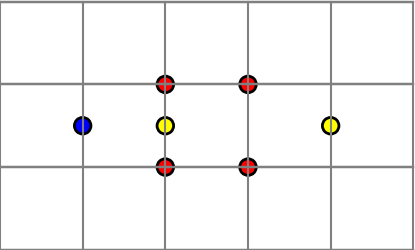
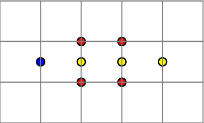
When you see a triangle made of two arrows, what’s the significance of the existence of an arrow that makes the diagram into a triangle? What difference does it make when the missing arrow goes on one side of the diagram or the other as in the two diagrams below?

The answer is not obvious if you’re unfamiliar with this way of thinking, and yet the problem has nothing to do with category theory per se. You could ask the question in the context of finite sets and functions. And that’s what Lawvere’s book does, acquainting the reader with diagrammatic reasoning before getting into category theory as such.

***

[1] Or more to the heart of the matter, you have definitions in terms of functions (“morphisms”) that are represented by diagrams. The difficulty does not come from the diagrams but rather from formulating things in terms of the existence and uniqueness of functions rather than more tangible arguments about sets and elements. This indirect formulation may seem unnecessary, or even sadistic, but it is generalizes further.

Simple example of Kleisli composition

Mars Climate Orbiter, artist conception, via NASA

When a program needs to work with different systems of units, it’s best to consistently use one system for all internal calculations and convert to another system for output if necessary. Rigidly following this convention can prevent bugs, such as the one that caused the crash of the Mars Climate Orbiter.

For example, maybe you need to work in degrees and radians. It would be sensible to do all calculations in radians, because that’s what software libraries expect, and output results in degrees, because that’s what humans expect.

Now suppose you have a function that takes in a length and doubles it, and another function takes in a length and triples it. Both functions take in length in kilometers but print the result in miles.

You would like the composition of the two functions to multiply a length by six. And as before, the composition would take in a speed in kilometers and return a speed in miles.

Here’s how we could implement this badly.

    miles_per_km = 5/8 # approx

    def double(length_km): 
        return 2*length_km*miles_per_km

    def triple(length_km): 
        return 3*length_km*miles_per_km

    length_km = 8
    d = double(length_km)
    print("Double: ", d)
    t = triple(d)
    print("Triple: ", t)

This prints

    Double: 10.0
    Triple: 18.75

The second output should be 30, not 18.5. The result is wrong because we converted from kilometers to miles twice. The correct implementation would be something like the following.

    miles_per_km = 0.6213712

    def double(length_km): 
        d = 2*length_km
        print("Double: ", d*miles_per_km)
        return d

    def triple(length_km): 
        t = 3*length_km
        print("Triple: ", t*miles_per_km)
        return t

    length_km = 8
    d = double(length_km)
    t = triple(d)

This prints the right result.

    Double: 10.0 
    Triple: 30.0

In abstract terms, we don’t want the composition of f and g to be simply gf.

We have a function f from X to Y that we think of as our core function, and a function T that translates the output. Say f doubles its input and T translates from kilometers to miles. Let f* be the function that takes X to TY, i.e. the combination of f and translation.

Now take another function g from Y to Z and define g* as the function that takes Y to TZ. We want the composition of f* and g* to be

g* ∘ f* = T ∘ g ∘ f.

In the example above, we only want to convert from kilometers to miles once. This is exactly what Kleisli composition does. (“Kleisli” rhymes with “highly.”)

Kleisli composition is conceptually simple. Once you understand what it is, you can probably think of times when it’s what you wanted but you didn’t have a name for it.

Writing code to encapsulate Kleisli composition takes some infrastructure (i.e. monads), and that’s a little complicated, but the idea of what you’re trying to achieve is not. Notice in the example above, what the functions print is not what they return; the print statements are a sort of side channel. That’s the mark of a monad.

Kleisli categories

The things we’ve been talking about are formalized in terms of Kleisli categories. You start with a category C and define another category that has the same objects as C does but has a different notion of composition, i.e. Kleisli composition.

Given a monad T on C, the Kleisli category CT has the same objects as C. An arrow f* from X to Y in CT corresponds to an arrow f from X to TY in C. In symbols,

HomCT(X, Y) = HomC(X, TY).

Mr. Kleisli’s motivation for defining his categories was to answer a more theoretical question—whether all monads arise from adjunctions—but more practically we can think of Kleisli categories as a way of formalizing a variation on function composition.

Related posts

Getting pulled back in

“Just when I thought I was out, they pull me back in.” — Michael Corleone, The Godfather, Part 3

My interest in category theory goes in cycles. Something will spark my interest in it, and I’ll dig a little further. Then I reach my abstraction tolerance and put it back on the shelf. Then sometime later something else comes up and the cycle repeats. Each time I get a little further.

A conversation with a client this morning brought me back to the top of the cycle: category theory may be helpful in solving a concrete problem they’re working on.

I’m skeptical of applied category theory that starts with categories. I’m more bullish on applications that start from the problem domain, a discussion something like this.

“Here’s a pattern that we’re trying to codify and exploit.”

“Category theory has a name for that, and it suggests you might also have this other pattern or constraint.”

“Hmm. That sounds plausible. Let me check.”

I think of category theory as a pattern description language, a way to turn vague analogies into precise statements. Starting from category theory and looking for applications is less likely to succeed.

When I left academia the first time, I got a job as a programmer. My first assignment was to make some change to an old Fortran program, and I started asking a lot of questions about context. My manager cut me off saying “You’ll never get here from there.” I had to work bottom-up, starting from the immediate problem. That lesson has stuck with me ever since.

Sometimes you do need to start from the top and work your way down, going from abstract to concrete, but less often that I imagined early in my career.

Galois connections and Galois theory

What are Galois connections and what do they have to do with Galois theory?

Galois connections are much more general than Galois theory, though Galois theory provided the first and most famous example of what we now call a Galois connection.

Galois connections

Galois connections are much more approachable than Galois theory. A Galois connection is just a pair of functions between partially ordered sets that have some nice properties. Specifically, let (A, ≤) and (B, ≤) be partially ordered sets. Here “≤” denotes the partial order on each set, and so could be defined differently on A and B.

We could add subscripts to distinguish the two meanings of ≤ but this is unnecessary because the meaning is always clear from context: if we’re comparing two things from A, we’re using the ≤ operator on A, and similarly for B.

Note that “≤” could have something to do with “less than” but it need not; it represents a partial order that may or may not be helpful to think of as “less than” or something analogous to less than such as “contained in.”

Monotone and antitone functions

Before we can define a Galois connection, we need to define monotone and antitone functions.

A monotone function is an order preserving function. That is, a function f is monotone if

xyf(x) ≤ f(y).

Similarly, an antitone function is order reversing. That is, a function f is antitone if

xy ⇔ f(x) ≥ f(y).

Here ≥ is defined by

yxxy.

Monotone and antitone connections

Galois connections have been defined two different ways, and you may run into each in different contexts. Fortunately it’s trivial to convert between the two definitions.

The first definition says that a Galois connection between A and B is a pair of monotone functions F and G such that for all a in A and b in B,

F(a) ≤ baG(b).

The second definition says that a Galois connection between A and B is a pair of antitone functions F and G such that for all a in A and b in B,

F(a) ≤ ba ≥ G(b).

If you need to specify which definition you’re working with, you can call the former a monotone Galois connection and the latter an antitone Galois connection. We only need one of these definitions: if we reverse the definition of ≤ on B then a monotone connection becomes antitone and vice versa. [1]

How can we just reverse the meaning of ≤ willy-nilly? Recall that we said above that ≤ is just a notation for a partial order. There’s no need for it to mean “less than” in any sense, and the opposite of a partial order is another partial order.

We’ll use the antitone definition for the rest of the post because our examples are antitone. Importantly, the Fundamental Theorem of Galois Theory involves an antitone connection.

Examples

For our first example, let A be sets of points in the plane, and let B be sets of lines in the plane. For both sets let ≤ mean subset.

For a set of points X, define F(X) to be the set of lines that go through all the points of X.

Similarly, for a set of lines Y, define G(Y) to be the set of points on all the lines in Y.

Then the pair (F, G) form a Galois connection.

This example can be greatly generalized. Let R be any binary relation between A and B and let ≤ mean subset.

Define

F(X) = { y | x R y for all x in X }

G(Y) = { x | x R y for all y in Y }

Then the pair (F, G) form a Galois connection. The example above is a special case of this construction where x R y is true if and only if x is a point on y. Garrett Birkhoff made this observation in 1940 [2].

Galois theory

Galois theory is concerned with fields, extension fields, and automorphisms of fields that keep a subfield fixed.

I recently wrote a series of blog posts explaining what images on the covers of math books were about, and one of these posts was an explanation of the following diagram:


Each node in the graph is a field, and a line means the field on the higher level is an extension of the field on the lower level. For each graph like this of extension fields, there is a corresponding graph of Galois groups. Specifically, let L be the field at the top of the diagram and let E be any field in the graph.

The corresponding graph of groups replaces E with the group of group isomorphisms from L to L that leave the elements of E unchanged, the automorphisms of L that fix E. This map from fields to groups is half of a Galois connection pair. The other half is the map that takes each group to the field of elements of L fixed by G. This connection is antitone because if a field F is an extension of E, then the group of automorphisms that fix F are a subgroup of the automorphisms that fix E.

***

[1] We could think of A and B as categories, where there is a morphism between x and y iff xy. Then a monotone Galois connection between A and B is an antitone Galois connection between A and Bop.

[2] Garrett Birkhoff. Lattice Theory. American Mathematical Society Colloquium Publications, volume 25. New York, 1940.