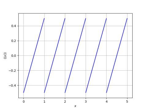
Sawtooth waves

I woke up around 3:00 this morning to some sort of alarm outside. It did not sound like a car alarm; it sounded like a sawtooth wave. The pattern was like a few Morse code O’s. Not SOS, or I would have gotten up to see if anyone needed help. Just O’s.

A sawtooth wave takes its name from the shape of its waveform: it looks like the edge of a saw. It also sounds a little jagged.

Sawtooth waves have come up several times here. For one thing, they have rich harmonics. Because the wave form is discontinuous, the Fourier coefficients decay to zero slowly. I wrote about that here. The post is about square waves and triangular waves, but sawtooth waves are very similar.

Here’s a post oscillators with a sawtooth forcing function.

I took sawtooth functions in a different direction in this post that started with an exercise from Knuth’s TAOCP. This led me down a rabbit hole on replicative functions and multiplication theorems in different contexts.

If I remember correctly the sound used for red alterts in Star Trek TOS started with a sawtooth wave. Early synthesizers had sawtooth generators because, as mentioned above, these waves are rich in overtones and can be manipulated to create interesting sounds such as the red alert sound.

Pitch of a big wine bottle

Yesterday my daughter came by and dropped off a huge blue wine bottle (empty).

Trader Joe's Incanto Chardonnay Pinot Grigio

She had started removing the label, but as you can see she didn’t get very far yet. It’s an Incanto Chardonnay Pinot Grigio from Trader Joe’s.

I blew across the top of the bottle to hear what sound it makes, and it makes a nice deep rumble.

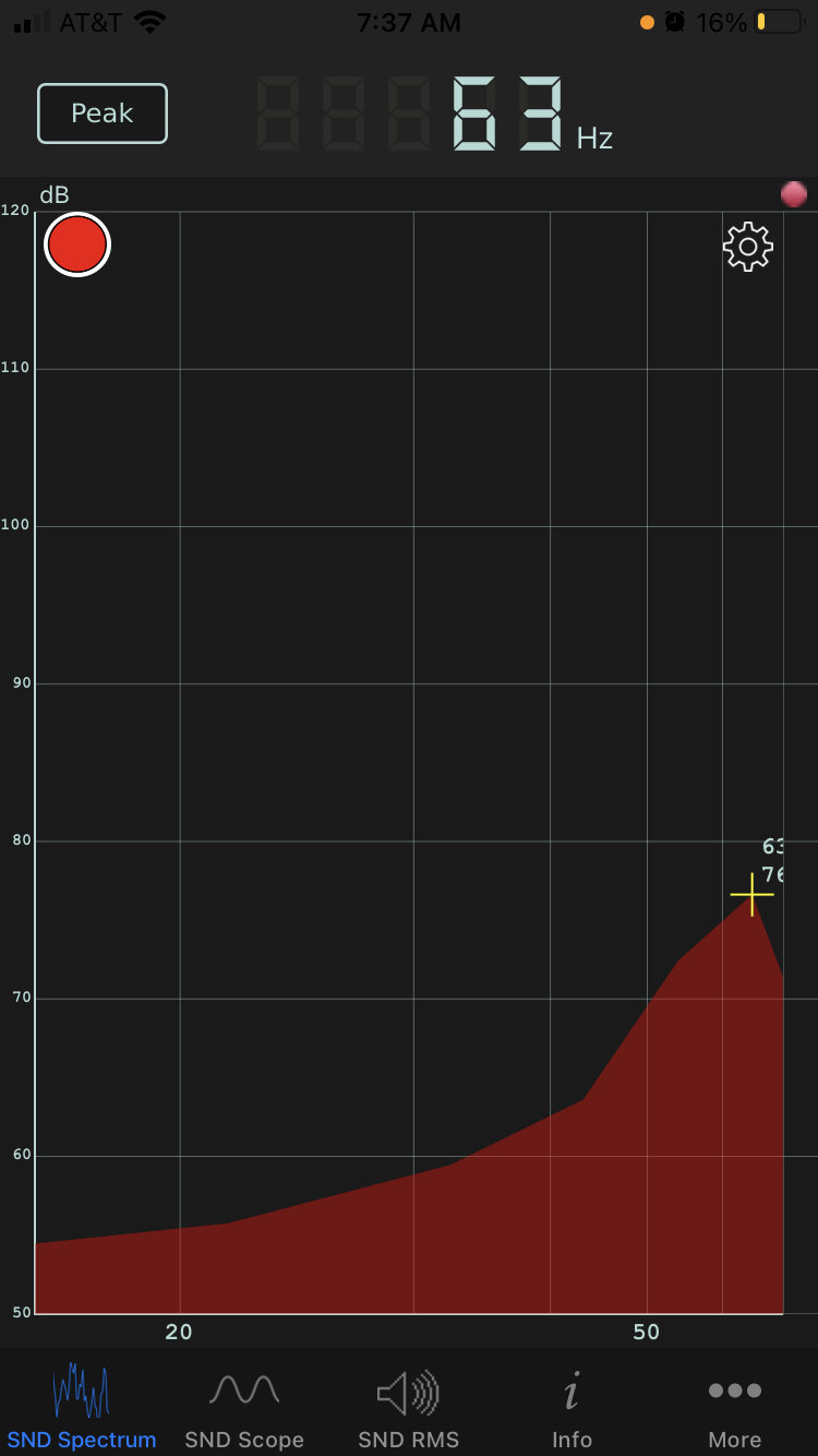
I tried to identify the pitch using a spectrum analyzer app on my phone, and it says 63 Hz.

audio spectrum analyzer screen shot

Next I tried to figure out what pitch I should expect theoretically based on physics. Wine bottles are Helmholtz resonators, and there’s a formula for the fundamental frequency of Helmholtz resonators:

f = \frac{v}{2\pi} \sqrt{\frac{A}{LV}}

The variables in this equation are:

  • f, frequency in Hz
  • v, velocity of sound
  • A, area of the opening
  • L, length of the neck
  • V, volume

I measured the opening to be 3/4 of an inch across, and the neck to be about 7 inches. The volume is 1.5 liters. The speed of sound at sea level and room temperature is 343 meters per second. After a few unit conversions [1] I got a result of 56.4 Hz, about 10% lower than what the spectrum analyzer measured.

An ideal Helmholtz resonator has a cylindrical neck attached to a spherical body. This bottle is far from spherical. The base is an ellipse with a major axis about twice as long as the minor axis. And from there it tapers off more like a cone than a sphere [2]. And yet the frequency predicted by Helmholtz’ formula comes fairly close to what I measured empirically.

I suspect I got lucky to some extent. I didn’t measure the bottle that accurately; it’s hard to even say when the neck of the bottle stops. But apparently Helmholtz’ formula is robust to changes in shape.

Update: Pitch of a beer bottle

I repeated my experiment with a beer bottle, specifically a Black Venom Imperial Stout.

Black Venom Imperial Stout

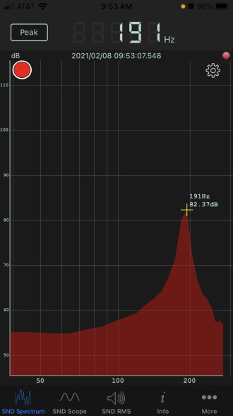
The opening diameter is about 3/4″, as with the wine bottle above, and the neck is about 3″ long. The volume is 12 fluid ounces. Helmholtz’ formula predicts a pitch of 177 Hz. My spectrum analyzer measured 191 Hz, the G below middle C. So this time theory was about 7% lower than the observed value.

Spectral analysis of blowing across beer bottle

The beer bottle is closer to the shape of a Helmholtz resonator than the wine bottle was. It’s at least radially symmetric, but the body is a cylinder rather than a sphere.

Update 2: Typical wine bottle

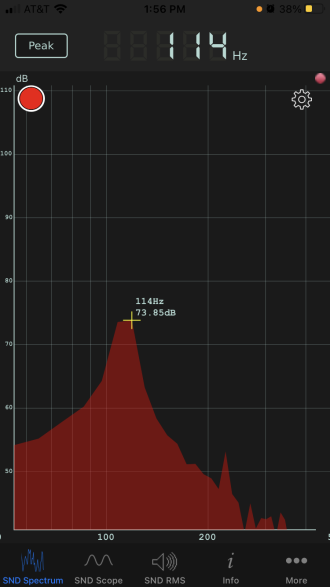
When I tested a typical 750 ml wine bottle, I got a pitch of 114 Hz. With a 3.5 inch neck and a 0.75 in diameter opening, the calculated pitch was 113 Hz. There’s some element of luck that theory and measurement agree so well, especially since the punt at the bottom means its shape is even further from spherical than that of a beer bottle.

Audio spectrum of a 750 ml pinot noir bottle

More acoustics posts

[1] Thanks to a reader who provided this write-up of the calculation:

calculation with dimensions

[2] What we usually call a cone is more specifically a right circular cone. But more generally a cone can have any base, not just a circle, and this bottle is approximately an elliptical cone.

Python and the Tell-Tale Heart

I was browsing through SciPy documentation this evening and ran across a function in scipy.misc called electrocardiogram. What?!

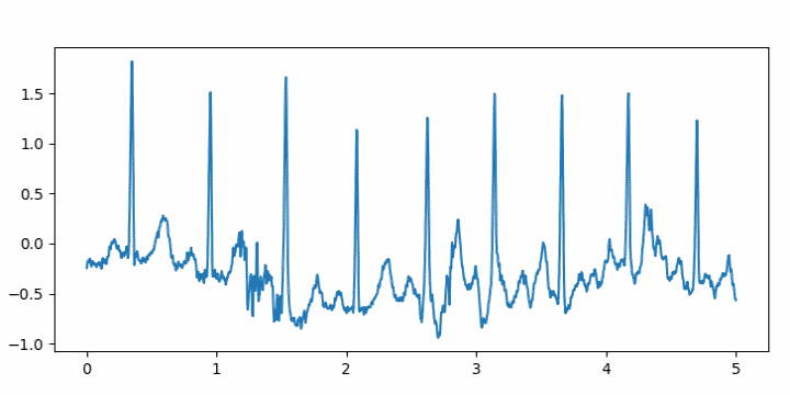
It’s an actual electrocardiogram, sampled at 360 Hz. Presumably it’s included as convenient example data. Here’s a plot of the first five seconds.

ECG plot

I wrote a little code using it to turn the ECG into an audio file.

from numpy import int16, iinfo
from scipy.io.wavfile import write
from scipy.misc import electrocardiogram

def to_integer(signal):
    # Take samples in [-1, 1] then scale to 16-bit integers
    m = iinfo(int16).max
    M = max(abs(signal))
    return int16(signal*m/M)

ecg = electrocardiogram()
write("heartbeat.wav", 360, to_integer(ecg))

I had to turn the volume way up to hear it, and that made me think of Edgar Allan Poe’s story The Tell-Tale Heart.

I may be doing something wrong. According to the documentation for the write function, I shouldn’t need to convert the signal to integers. I should just be able to leave the signal as floating point and normalize it to [−1, 1] by dividing by the largest absolute value in the signal. But when I do that, the output file will not play.

Related posts

Updated pitch calculator

I’ve made a couple minor changes to my page that converts between frequency and pitch. (The page also includes Barks, a psychoacoustic unit of measure.)

If you convert a frequency in Hertz to musical notation, the page used to simply round to the nearest note in the chromatic scale. Now the page will also tell you how sharp or flat the pitch is if it’s not exact.

For example, if you enter 1100 Hz, the page used to report simply “C#6” and now it reports “C#6 − 14 cents” meaning the closest note is C#6, but it’s a little flat, 14/100 of a semitone flat. If you enter 1120 Hz it will report “C#6 + 18 cents” meaning that the note is 18/100 of a semitone sharp.

Octave numbers, such as the 6 in C#6 are explained here.

The other change I made to the page was to add a little eighth note favicon that might show up in a browser tab.

pitch converter favicon

I’ve written several online converters like this: LaTeX to Unicode, wavelength to RGB, etc. See a full list here.


Determining fundamental frequency

My daughter had a homework problem the other day that gave the frequencies of several Fourier components and asked her to find the fundamental frequency. The numbers were nice enough that brute force worked, and I’m sure that’s what students were expected to do. But this could easily be a much more sophisticated problem.

If the frequencies are all integers and exact multiples of a fundamental frequency, you can simply take the greatest common divisor of the frequencies. If you’re told the frequencies are 1760, 2200, and 3080, then the fundamental frequency is apparently 440 since that’s the greatest common divisor.

But what if the data are a little different? Say the highest pitch is 3081. Surely 440 should still be considered the fundamental frequency, even though now the greatest common divisor of the frequencies would be 1 Hz. What if the highest frequency was 3078 + π? Surely the fundamental frequency is still 440 for practical purposes.

And what might these practical purposes be? One purpose might be pitch detection. When several frequencies are combined that are small integer multiples of a fundamental frequency, we perceive the combination as having pitch given by that fundamental.

For something like a guitar string, the frequency components are close to small integer multiples of a fundamental frequency. But for something like a church bell, the frequencies don’t line up so neatly, though there’s still a clearly perceived pitch. For something like a metal mixing bowl, it may be difficulty to predict what pitch a person will hear when something strikes the bowl.

One complication we haven’t addressed yet is that the fundamental frequency will not be unique without some constraint. In the example above, the frequencies were all multiples of 440, but they’re also all multiples of 440/n for every positive integer n. We might get around this by specifying some lower bound on the fundamental frequency. Or we could say that all other things being equal, we want the largest candidate for the fundamental frequency.

We could formulate the problem of finding the fundamental frequency as an optimization problem. For example, we could form a mixed integer program. Suppose we have three frequencies f1, f2, and f3. We could find a fundamental frequency f and integers n1, n2, and n3 that minimize

(f1n1 f)² + (f2n2 f)² + (f3n3 f

subject to a lower bound on f.

We can eliminate the explicit dependence on the integer coefficients by minimizing

(f1/f − [f1/f])² + (f2/f − [f2/f])² + (f3/f − [f3/f])² .

where [x] denotes nearest integer to x. The first formulation has a more common form. The latter has a more complicated objective function, but it’s only a function of one variable.

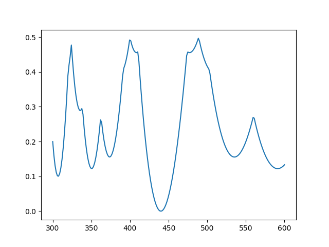
Here’s what the latter looks like for frequencies 1760, 2200, and 3080.

objective function

Clearly there’s a minimum at 440 Hz.

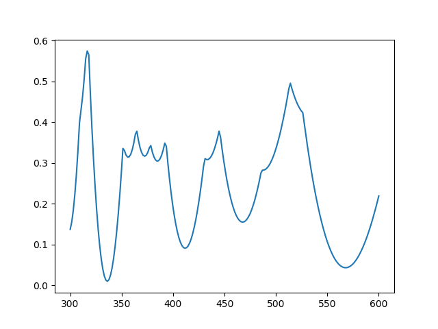
Here’s the same plot with 10% random noise [1] added to each frequency: 1701, 2368, and 3339.

objective function

Now there’s a minimum near 336, but the local minimum at 566 is nearly as good.

Related posts

[1] There are a couple reasons you might want to solve a problem like this. Maybe your frequencies really are integer multiples of a fundamental frequency, but there is measurement error. Another is that the frequencies are not exactly multiples of a fundamental, as when striking a bell or a mixing bowl. How might you formulate the two cases differently?

The acoustics of Hagia Sophia

Hagia Sophia

The Hagia Sophia (Greek for “Holy Wisdom”) was a Greek Orthodox cathedral from 537 to 1453. When the Ottoman Empire conquered Constantinople the church was converted into a mosque. Then in 1935 it was converted into a museum.

No musical performances are allowed in the Hagia Sophia. However, researchers from Stanford have modeled the acoustics of the space in order to simulate what worship would have sounded like when it was a medieval cathedral. The researchers recorded a virtual performance by synthesizing the acoustics of the building. Not only did they post-process the sound to give the singers the sound of being in the Hagia Sophia, they first gave the singers real-time feedback so they would sing as if they were there.

Related posts

Mathematics of Deep Note

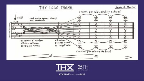
THX deepnote logo score

I just finished listening to the latest episode of Twenty Thousand Hertz, the story behind “Deep Note,” the THX logo sound.

There are a couple mathematical details of the sound that I’d like to explore here: random number generation, and especially Pythagorean tuning.

Random number generation

First is that part of the construction of the sound depended on a random number generator. The voices start in a random configuration and slowly reach the target D major chord at the end.

Apparently the random number generator was not seeded in a reproducible way. This was only mentioned toward the end of the show, and a teaser implies that they’ll go more into this in the next episode.

Pythagorean tuning

The other thing to mention is that the final chord is based on Pythagorean tuning, not the more familiar equal temperament.

The lowest note in the final chord is D1. (Here’s an explanation of musical pitch notation.) The other notes are D2, A2, D3, A3, D4, A4, D5, A5, D6, and F#6.

Octaves

Octave frequencies are a ratio of 2:1, so if D1 is tuned to 36 Hz, then D2 is 72 Hz, D3 is 144 Hz, D4 is 288 Hz, D5 is 576 Hz, and D6 is 1152 Hz.

Fifths

In Pythagorean tuning, fifths are in a ratio of 3:2. In equal temperament, a fifth is a ratio of 27/12 or 1.4983 [1], a little less than 3/2. So Pythagorean fifths are slightly bigger than equal temperament fifths. (I explain all this here.)

If D2 is 72 Hz, then A2 is 108 Hz. It follows that A3 would be 216 Hz, A4 would be 432 Hz (flatter than the famous A 440), and A5 would be 864 Hz.

Major thirds

The F#6 on top is the most interesting note. Pythagorean tuning is based on fifths being a ratio of 3:2, so how do you get the major third interval for the highest note? By going up by fifths 4 times from D4, i.e. D4 -> A4 -> E5 -> B5 -> F#6.

The frequency of F#6 would be 81/16 of the frequency of D4, or 1458 Hz.

The F#6 on top has a frequency 81/64 that of the D# below it. A Pythagorean major third is a ratio of 81/64 = 1.2656, whereas an equal temperament major third is f 24/12 or 1.2599 [2]. Pythagorean tuning makes more of a difference to thirds than it does to fifths.

A Pythagorean major third is sharper than a major third in equal temperament. Some describe Pythagorean major chords as brighter or sweeter than equal temperament chords. That the effect the composer was going for and why he chose Pythagorean tuning.

Detuning

Then after specifying the exact pitches for each note, the composer actually changed the pitches of the highest voices a little to make the chord sound fuller. This makes the three voices on each of the highest notes sound like three voices, not just one voice. Also, the chord shimmers a little bit because the random effects from the beginning of Deep Note never completely stop, they are just diminished over time.

Related posts


[1] The exponent is 7/12 because a half step is 1/12 of an octave, and a fifth is 7 half steps.

[2] The exponent is 4/12 because a major third is 4 half steps.

Musical score above via THX Ltd on Twitter.
Generating pink noise

Different colors of noise are named by analogy with colors of light. Pink noise is between white noise and red noise.

White noise has equal power at all frequencies, just as white light is a combination of all the frequencies of the visible spectrum. The components of red noise are weighted toward low frequencies, just as red light is at the low end of the visible spectrum. Pink noise is weighted toward low frequencies too, but not as strongly as red. Specifically, the power in red noise drops off like 1/f² where f is frequency. The power in pink noise drops off like 1/f.

Generating pink noise is more complicated than you might think. The book Creating Noise, by Stefan Hollos and J. Richard Hollos, has a good explanation and C source code for generating pink noise and variations such as 1/f α noise for 0 < α < 1. If you want even more background, check out Recursive Digital Filters by the same authors.

If you’d like to hear what pink noise sounds like, here’s a sample that was created using the software in the book with a 6th order filter.

(Download)

More posts on noise

Acoustic roughness examples

Amplitude modulated signals sound rough to the human ear. The perceived roughness increases with modulation frequency, then decreases, and eventually disappears. The point where roughness reaches is maximum depends on the carrier signal, but for a 1 kHz tone roughness reaches a maximum for modulation at 70 Hz. Roughness also increases as a function of modulation depth.

Amplitude modulation multiplies a carrier signal by

1 + d sin(2π f t)

where d is the modulation depth, f is the modulation frequency, and t is time.

Here are some examples you can listen to. We use a pure 1000 Hz tone and Gaussian white noise as carriers, and vary modulation depth and frequency continuously over 10 seconds. he modulation depth example varies depth from 0 to 1. Modulation frequency varies from 0 to 120 Hz.

First, here’s a pure tone with increasing modulation depth.


Next we vary the modulation frequency.


Now we switch over to Gaussian white noise, first varying depth.


And finally white noise with varying modulation frequency. This one sounds like a prop-driven airplane taking off.


Related: Psychoacoustics consulting

Quantifying how annoying a sound is

leaf blower

Eberhard Zwicker proposed a model for combining several psychoacoustic metrics into one metric to quantify annoyance. It is a function of three things:

  • N5, the 95th percentile of loudness, measured in sone (which is confusingly called the 5th percentile)
  • ωS, a function of sharpness in asper and of loudness
  • ωFR, fluctuation strength (in vacil), roughness (in asper), and loudness.

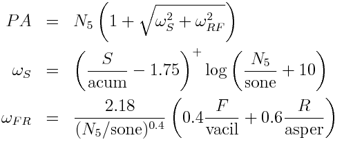
Specifically, Zwicker calculates PA, psychoacoutic annoyance, by

PA &=&N_5 \left( 1 + \sqrt{\omega_S^2 + \omega_{RF}^2}\right) \\ \omega_S &=& \left(\frac{S}{\mbox{acum}} - 1.75\right)^+ \log \left(\frac{N_5}{\mbox{sone}} + 10\right) \\ \omega_{FR} &=& \frac{2.18}{(N_5/\mbox{sone})^{0.4}} \left( 0.4 \frac{F}{\mbox{vacil}} + 0.6 \frac{R}{\mbox{asper}}\right)

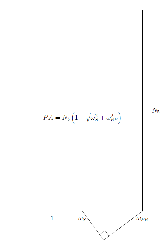
A geometric visualization of the formula is given below.

Geometric representation of Zwicker's annoyance formula

Here’s an example of computing roughness using two sound files from previous posts, a leaf blower and a simulated kettledrum. I calibrated both to have sound pressure level 80 dB. But because of the different composition of the sounds, i.e. more high frequency components in the leaf blower, the leaf blower is much louder than the kettledrum (39 sone vs 15 sone) at the same sound pressure level. The annoyance of the leaf blower works out to about 56 while the kettledrum was only about 19.