Partitioning complexity

This post looks at how to partition complexity between definitions and theorems, and why it’s useful to be able to partition things more than one way.

Quadratic equations

Imagine the following dialog in an algebra class.

“Quadratic equations always have two roots.”

“But what about (x − 5)² = 0. That just has one root, x = 5.”

“Well, the 5 counts twice.”

Bézout’s theorem

Here’s a more advanced variation on the same theme.

“A curve of degree m and a curve of degree n intersect in mn places. That’s Bézout’s theorem.”

“What about the parabola y = (x − 5)²  and the line y = 0. They intersect at one point, not two points.”

“The point of intersection has multiplicity two.”

“That sounds familiar. I think we talked about that before.”

“What about the parabola y = x² + 1 and the line y = 0. They don’t intersect at all.”

“You have to look at complex numbers. They intersect at x = i and x = −i.”

“Oh, OK. But what about the line y = 5 and the line y = 6. They don’t intersect, even for complex numbers.”

“They intersect at the point at infinity.”

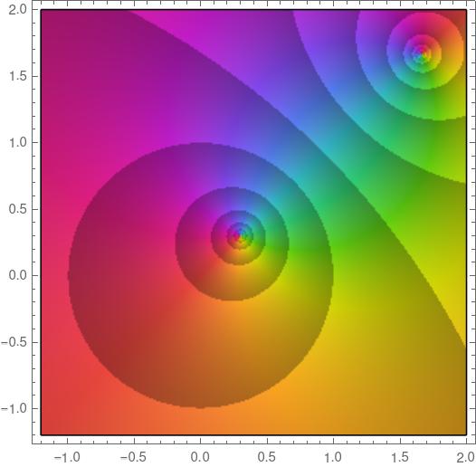
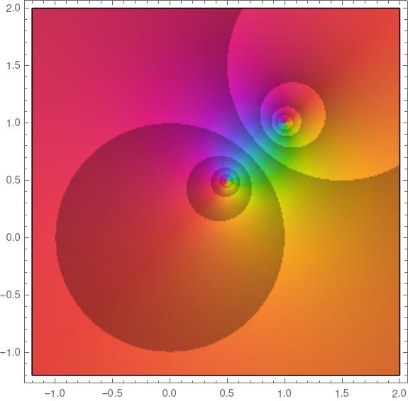
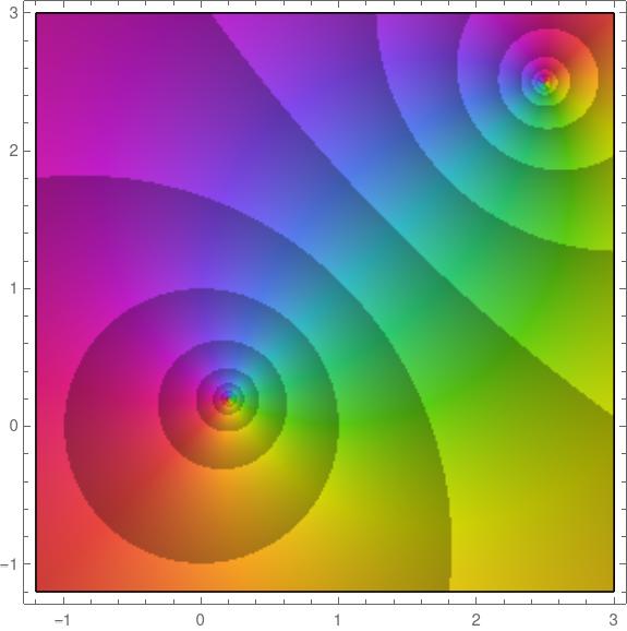
In order to make the statement of Bézout’s theorem simple you have to establish a context that depends on complex definitions. Technically, you have to work in complex projective space.

Definitions and theorems

Michael Spivak says in the preface to his book Calculus on Manifolds

… the proof of [Stokes’] theorem is … an utter triviality. On the other hand, even the statement of this triviality cannot be understood without a horde of definitions … There are good reasons why the theorems should all be easy and the definitions hard.

There are good reasons, for the mathematician, to make the theorems easy and the definitions hard. But for students, there may be good reasons to do the opposite.

Here math faces a tension that programming languages (and spoken languages) face: how to strike a balance between the needs of novices and the needs of experts.

In my opinion, math should be taught bottom-up, starting with simple definitions and hard theorems, valuing transparency over elegance. Then, motivated by the complication of doing things the naive way, you go back and say “In light of what we now know, let’s go back and define things differently.”

It’s tempting to think you can save a lot of time by starting with the abstract final form of a theory rather than working up to it. While that’s logically true, it’s not pedagogically true. A few people with an unusually high abstraction tolerance can learn this way, accepting definitions without motivation or examples, but not many. And the people who do learn this way may have a hard time applying what they learn.

Applications

Application requires moving up and down levels of abstraction, generalizing and particularizing. And particularizing is harder than it sounds. This lesson was etched into my brain by an incident I relate here. Generalization can be formulaic, but recognizing specific instances of more general patterns often requires a flash of insight.

Spivak said there are good reasons why the theorems should all be easy and the definitions hard. But I’d add there are also good reasons to remember how things were formulated with hard theorems and easy definitions.

It’s good, for example, to understand analysis at a high level as in Spivak’s book, with all the machinery of differential forms etc. and also be able to swoop down and grind out a problem like a calculus student.

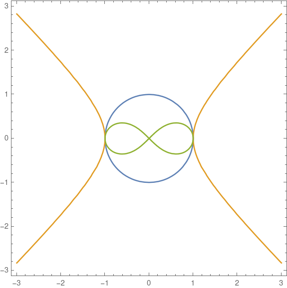
Going back to Bézout’s theorem, suppose you need to find real solutions a system of equations that amounts to finding where a quadratic and cubic curve intersect. You have a concrete problem, then you move up to the abstract setting of Bézout’s theorem learn that there are at most six solutions. Then you go back down to the real world (literally, as in real numbers) and find two solutions. Are there any more solutions that you’ve overlooked? You zoom back up to the abstract world of Bézout’s theorem, and find four more by considering multiplicities, infinities, and complex solutions. Then you go back down to the real world, satisfied that you’ve found all the real solutions.

A pure mathematician might climb a mountain of abstraction and spend the rest of his career there, but applied mathematicians have to go up and down the mountain routinely.

French palindromes and Morse code

I got an email from a student in France who asked about a French counterpart to my post on Morse code palindromes, and this post is a response to that email.

Palindromes

A palindrome is a word that remains the same when the letters are reversed, like kayak. A Morse code palindrome is a word that remains the same when its Morse code representation is reversed.

The word kayak is not a Morse code palindrome because its Morse code representation

    -.- .- -.-- .- -.-

when reversed becomes

    -.- -. --.- -. -.-

which is the Morse code for knqnk.

The word wig is a palindrome in Morse code because

    .-- .. --.

reads the same in reverse.

French distinctives

Now what about French? I saved the script I wrote to find Morse palindromes in English, and I ran it on the French dictionary located at

    /usr/share/dict

on my Linux box.

I thought I’d have to modify the script because French uses characters in addition to the 26 letters of the Roman alphabet, such as ç, a ‘c’ with a cedilla. There is a Morse code for ç

    -.-..

but its reverse is not a letter.

It’s not clear exactly what is “French Morse code” because there are a number of code values that could be used in French (or English) to represent letters with diacritical marks.

The code for é is itself a palindrome, so I didn’t need to modify my script for it. As far as I know, there are no codes for accented letters which are valid letters when reversed, except for ü whose code is the opposite of z. But there are no Morse palindromes in French if you add ü.

Results

See this file for complete results. Some of these words remain the same when translated to Morse, reversed, and translated back, such as sans. Others, are pairs that of valid words but not the same word, such as ail and fin.

Related posts

Blaschke factors

Blaschke factors are complex functions with specified zeros inside the unit disk. Given a complex number a with |a| < 1, the Blaschke factor associated with a is the function

b(z; a) = \frac{|a|}{a} \frac{a-z}{1 -\bar{a}z}

Notice the semicolon in b(z; a). This is a convention that a few authors follow, and that I wish more would adopt. From a purely logical perspective the semicolon serves no purpose because the expression on the right is a function of two variables, z and a. But the semicolon conveys how we think about the function: we think of it as a function of z that depends on a parameter a.

So, for example, if we were to speak of the derivative of b, we would mean the derivative with respect to z. And we could say that that b is an analytic function inside the unit disk. It is not an analytic function if we think of it as a function of a because of taking the conjugate of a in the denominator.

The function b(z; a) has a zero at a and a pole at the reciprocal of the conjugate of a. So, as I wrote about yesterday, this means that the zero and the pole are inversions of each other in the unit circle. If you punch a hole in the complex plane at the origin and turn the plane inside-out, without moving the unit circle, the zero and pole will swap places.

Here’s a plot of b(z; 0.3 + 0.3i).

Notice there’s a zero at 0.3 + 0.3i and a pole at

1/(0.3 – 0.3i) = 5/3 + 5/3i

which is the inversion of 0.3 + 0.3i in the unit circle. You can tell that one is a zero and the other is a pole because the colors rotate in opposite directions.

The plot above was made with the following Mathematica code.

    b[z_, a_] := (Abs[a]/a) (a - z)/(1 - Conjugate[a] z)
    ComplexPlot[b[z, .3 + .3 I], {z, -1.2 - 1.2 I, 2 + 2 I}, 
        ColorFunction -> "CyclicLogAbs"]

Because the zero and pole locations are inversions of each other, as the zero moves closer to the unit circle from the inside, the pole moves closer to the unit circle from the outside. Here’s a plot with a = 0.5 + 0.5i.

And the closer the zero gets to the origin, the further out the pole moves. Here’s a plot with a = 0.2 + 0.2i, this time on a larger scale, this time with the real and imaginary axes going up to 3 rather than 2.

Blaschke factors are the building blocks of Blaschke products, something I intend to write about in the future. By multiplying Blaschke factors together, you can create function that is analytic in the unit disk with specified zeros and with other nice properties.

Elias Wegert [1] says “In some sense, Blaschke products can be considered to be ‘hyperbolic counterparts’ of polynomials.” That’s something I’d like to explore further.

Related posts

[1] Elias Wegert. Visual Complex Functions: An Introduction with Phase Portraits. Birkhäuser.

Inversion in a circle

Inversion in the unit circle is a way of turning the circle inside-out. Everything that was inside the circle goes outside the circle, and everything that was outside the circle comes in.

Not only is the disk turned inside-out, the same thing happens along each ray going out from the origin. Points on that ray that are inside the circle go outside and vice versa. In polar coordinates, the point (r, θ) goes to (1/r, θ).

Complex numbers

In terms of complex numbers, inversion in the unit circle amounts to taking the reciprocal and the conjugate (in either order, because these operations commute). This is the same as dividing a complex number by the square of its magnitude. Proof:

z \bar{z} = |z|^2 \implies \frac{1}{\bar{z}} = \frac{z}{|z|^2}

There are two ways to deal with the case z = 0. One is to exclude it, and the other is to say that it maps to the point at infinity. This can be made rigorous by working on the Riemann sphere rather than the complex plane. More on that here.

Inverting a hyperbola

The other day Alex Kantorovich pointed out on Twitter that “the perfect figure 8 (or infinity) is simply the inversion through a circle of a hyperbola.” We’ll demonstrate this with Mathematica.

What happens to a point on the hyperbola

x^2 - y^2 = 1

when you invert it through a circle? If we think of x and y as the real and imaginary parts of a complex number, the discussion above shows that the point (x, y) goes to the same point divided by its length squared.

(x, y) \mapsto \left( \frac{x}{x^2 + y^2}, \frac{y}{x^2 + y^2} \right)

Let (u, v) be the image of the point (x, y).

\begin{align*} u &= \frac{x}{x^2 + y^2} \\ v &= \frac{y}{x^2 + y^2} \end{align*}

Then we have

u^2 + y^2 = \frac{x^2 + v^2}{(x^2 + y^2)^2} = \frac{1}{x^2 + y^2}

and

u^2 - v^2 = \frac{x^2 - y^2}{(x^2 + y^2)^2} = \frac{1}{(x^2 + y^2)^2}

because x² − y² = 1. Notice that the latter is the square of the former, i.e.

u^2 - v^2 = (u^2 + v^2)^2

Now we have everything to make our plot. The code

ContourPlot[{
    x^2 + y^2 == 1, 
    x^2 - y^2 == 1, 
    x^2 - y^2 == (x^2 + y^2)^2}, 
    {x, -3, 3}, {y, -3, 3}]

produces the following plot.

The blue circle is the first contour, the orange hyperbola is the second contour, and the green figure eight is the third contour.

Related posts

How flat is a normal mixture on top?

Male and female heights both have a standard deviation of about 3 inches, with means of 70 inches and 64 inches. That’s a good first-pass model using round numbers.

If you ask what the height of an average adult is, not specifying male or female, you get a mixture of two normal distributions. If we assume an equal probability of selecting a male or female, then the probability density function for the mixture is the average of the density functions for men and women separately.

This mixture distribution is remarkably flat on top.

This happens whenever you have an equal mixture of two normal distributions, both having the same standard deviation σ, and with means 2σ apart. If the means were any closer together, the distribution would be rounder on top. If the means were any further apart, there would be a dip in the middle.

This makes sense intuitively if you think about what happens if you make things more extreme. If the means were as close together as possible, i.e. if they were the same, we’d simply have a normal distribution with its familiar curve on top. If the means were much further apart, we’d have two bumps that hardly appear to overlap.

See more on the application to heights here.

Mathematical details

How flat is the mixture density on top? We can quantify the flatness by looking at a power series expansion centered at the peak.

To simplify matters, we can assume that σ = 1 and that the means of the two distributions are −μ and μ, with the primary interest being the case μ = 1. The probability density function for the mixture is

\frac{1}{2\sqrt{2\pi}}\left( \exp\left(\frac{-(x-\mu)^2}{2} \right ) + \exp\left(\frac{-(x+\mu)^2}{2} \right )\right )

If we expand this in a Taylor series around 0 we get

\exp\left( -\frac{\mu^2}{2} \right) \left( \frac{1}{2 \pi }+\frac{\left(\mu^2-1\right) x^2}{4 \pi }+\frac{ \left(\mu^4-6 \mu^2+3\right) x^4}{48 \pi } + \cdots \right)

This is a little complicated, but it explains a lot. Notice that the coefficient of x² has a term (μ² − 1).

We said above that if the means were any closer together than two standard deviations, the distribution would be rounder on top. That’s because if μ < 1 then (μ² − 1) is negative and the curve is convex on top.

We also said that if the means were any further apart, there would be a dip in the middle. That’s because if μ > 1 then (μ² − 1) is positive and the curve is concave on top.

Now if μ = 1 then the x² term disappears. And because our function is even, its Taylor series only has terms with even powers. So if the x² term goes away the next term is not x3 but x4.

So one way to say how flat our curve is on top is that it is flat to within O(x4).

Let’s get more specific by evaluating the coefficients numerically. For small x, our mixture density function is

0.0965 − 0.0080 x4 + O(x6).

Now if x is small, x4 is extremely small, and the coefficient of 0.008 makes it even smaller.

Hilbert transform and Fourier series

A few days ago I wrote about the Hilbert transform and gave as an example that the Hilbert transform of sine is cosine. We’ll bootstrap that example to find the Hilbert transform of any periodic function from its Fourier series.

The Hilbert transform of a function f(t) is a function fH(x) defined by

f_H(x) = \frac{1}{\pi} \int_{-\infty}^\infty \frac{f(t)}{t - x}\, dt

where the integral is interpreted in the sense of the Cauchy principal value, the limit as the singularity is approach symmetrically from both sides.

The Hilbert transform shifts and scales conveniently. Shifting a function by any amount h shifts its transform by the same amount. And scaling a function by any amount k > 0 scales its transform the same way. That is, we have the following transform pairs.

\begin{align*} f(t) &\leftrightarrow f_H(x) \\ f(t - h) &\leftrightarrow f_H(x - h) \\ f(kt) &\leftrightarrow f_H(kx) \\ \end{align*}

Now since the Hilbert transform of sin(t) is cos(x), the Hilbert transform of sin(t + π/2) must be cos(x + π/2). But sin(t + π/2) is cos(t), and cos(x + π/2) is sin(x), so the Hilbert transform of cos(t) is −sin(x). In this case, the Hilbert transform has the same pattern as differentiation.

Now if ω > 0 the scaling rule tells us the Hilbert transform of sin(ωt) is cos(ωx) and the Hilbert transform of cos(ωx) is −sin(ωx). Here the analogy with differentiation breaks down because differentiation would bring out a factor of ω from the chain rule [1].

Putting these facts together, if we have a function f written in terms of a Fourier series

f(t) = \sum_{n=1}^\infty \left\{ a_n \sin(nt) + b_n\cos(nt) \right\}

then its Hilbert transform is

f_H(x) = \sum_{n=1}^\infty \left\{ -b_n \sin(nx) + a_n\cos(nx) \right\}

In other words, we replace the b‘s with a‘s and the a‘s with −b‘s. [2]

Notice that there’s no b0 term above. In signal processing terminology, there’s no DC offset. In general a Fourier series has a constant term, and the Hilbert transform of a constant is 0. So again like differentiation, constants go away.

If there is no DC offset, then applying the Hilbert transform to f twice gives −f. If there is a DC offset, applying the Hilbert transform to f twice gives −f with the DC offset removed.

Opposite sign convention

Unfortunately there are two definitions of the Hilbert transform in common use: the one at the top of this post and its negative. What changes if we use the other convention?

We noted above that applying the Hilbert transform to f twice gives −f. This means that the inverse transform is the negative transform [3]. In symbols, if H is the Hilbert transform operator, then −H²f = −Hf and so H−1 = −H. So the disagreement over whether to include a negative sign in the definition of the Hilbert transform amounts to a disagreement over which to call the forward transform and which to call the inverse transform.

The shifting and scaling rules apply to both definitions of the transform. But with the opposite sign convention, the Hilbert transform of sine is negative cosine and the Hilbert transform of cosine is sine. So our bottom line becomes “replace the a‘s with b‘s and the b‘s with −a‘s” in the Fourier series.

Footnotes

[1] Incidentally, the Hilbert transform commutes with differentiation. That is, the transform of the derivative is the derivative of the transform.

[2] This is an example of parallel replacement. We replace an, with –bn and bn, with an at the same time.

[3] For signals with no DC offset. Otherwise the Hilbert transform is not invertible.

Logarithms yearning to be free

I got an evaluation copy of The Best Writing on Mathematics 2021 yesterday. One article jumped out as I was skimming the table of contents: A Zeroth Power Is Often a Logarithm Yearning to Be Free by Sanjoy Mahajan. Great title.

There are quite a few theorems involving powers that have an exceptional case that involves a logarithm. The author opens with the example of finding the antiderivative of xn. When n ≠ −1 the antiderivative is another power function, but when n = −1 it’s a logarithm.

Another example that the author mentions is that the limit of power means as the power goes to 0 is the geometric mean. i.e. the exponential of the mean of the logarithms of the arguments.

I tried to think of other examples where this pattern pops up, and I thought of a couple related to entropy.

q-logarithm entropy

The definition of q-logarithm entropy takes Mahajan’s idea and runs it backward, turning a logarithm into a power. As I wrote about here,

The natural logarithm is given by

\ln(x) = \int_1^x t^{-1}\,dt

and we can generalize this to the q-logarithm by defining

\ln_q(x) = \int_1^x t^{-q}\,dt

And so ln1 = ln.

Then q-logarithm entropy is just Shannon entropy with natural logarithm replaced by q-logarithm.

Rényi entropy

Quoting from this post,

If a discrete random variable X has n possible values, where the ith outcome has probability pi, then the Rényi entropy of order α is defined to be

H_\alpha(X) = \frac{1}{1 - \alpha} \log_2 \left(\sum_{i=1}^n p_i^\alpha \right)

for 0 ≤ α ≤ ∞. In the case α = 1 or ∞ this expression means the limit as α approaches 1 or ∞ respectively.

When α = 1 we get the more familiar Shannon entropy:

H_1(X) = \lim_{\alpha\to1} H_\alpha(X) = - \left(\sum_{i=1}^n p_i \log_2 p_i \right)

In this case there’s already a logarithm in the definition, but it moves inside the parentheses in the limit.

And if you rewrite

pα

as

p pα−1

then as the exponent in pα−1 goes to zero, we have a logarithm yearning to be free.

Related

Circular slide rule

I explained the basics of how a slide rule works in the previous post. But how does a circular slide rule work?

Mr. Spock holding an E6B circular slide rule

Apparently the prop Mr. Spock is holding is an E6B aircraft slide rule. It includes a circular slide rule and more functionality.

Start with an ordinary straight slide rule, with each bar labeled 1 on the left and 10 on the right end. Now imagine bending this into a circle so that you now have two concentric circles. For x between 1 and 10, the label for x is located at

log10 x × 360°.

Suppose you want to multiply x and y, and xy is less than 10, i.e. log10 x + log10 y < 1. Then the multiplication procedure works exactly analogously to how it would have with a straight slide rule. Line up the 1 of the inner ring with the position of x on the outer ring. The position of y on the inner ring lines up with xy on the outer ring because it is at position

log10 x × 360° + log10 y × 360° = log10 xy × 360°.

But what if xy > 10, i.e. log10 x + log10 y > 1? In that case the y on the inner ring is at position

(log10 x + log10 y) × 360°− 360° = (log10 x + log10 y − 1) × 360°

which is equal to

(log10 x + log10 y − log10 10) × 360° = log10 (xy/10) × 360°

and so the y on the inner ring is aligned with the position labeled xy/10. As we noted in the previous post, slide rules only give you the significand (mantissa) of the result, so a slide rule doesn’t know the difference between xy and xy/10. That’s up to you to keep up with.

E6B Flight Computer

Update: After first posting this article, I bought an E6B flight computer from Amazon for about $14. I bought the paper version because I’m certainly not going to wear it out. But if you’d like a nicer one, they make the same product in metal.

Here’s a photo of mine:

E6B analog flight computer

You can slide the horizontal piece out and essentially have a circular slide rule with some extra markings.

Why a slide rule works

Suppose you have two sticks. The length of one is log x, and the length of the other is log y. If you put the two sticks end to end, the combined length is

log x + log y = log xy.

That’s the basic idea behind a slide rule.

The simplest slide rule consists of two bars with numbers marked on each bar on a logarithmic scale, running from 1 to 10 or maybe 1 to 100.

To multiply x by y, line the 1 on the left end of the bottom bar with x on the top bar. Then the number above y on the bottom bar is xy on the top bar.

This works because the 1 of the bottom bar is positioned a distance log x from the 1 on the top bar. The y on the bottom bar is a distance log y further to the right, and so it is a distance log x + log y from the 1 on the top, which is marked with log xy.

Here’s an example. Suppose you want to find the circumference of a circle 5000 ft in diameter. The image below shows how you would multiply π times 5000.

Notice that the 1 of the bottom is under π on the top bar. The red hairline helps us see just where the five on the bottom scale lines up with the top scale, and that’s at about 15.8. Slide rules will only give you the significand (mantissa) of your product, so you have to know that your result is 15,800 ft.

(The lack of exponents could be a pedagogical feature rather than a bug. A few days of using a slide rule would make students think a little harder about what a reasonable answer should be, and would cure them of reporting a ridiculous amount of extraneous precision.)

It’s also possible to line the 10 (or 100) of the right end of the bottom scale with the x value on the top scale.

In the image above, I’ve lined the 100 of the bottom scale with 31.4 (10π) on the top scale. We’re only after the significand, so we’ll toss around factors of 10 willy nilly. The number above the 50 on the lower scale is about 15.6 on the upper scale. So this time we’d get an answer of about 15,600 ft. You can see right away that you’re going to need to be more careful, or preferably have a larger slide rule, if you want to get three or four significant figures.

The second example takes a little more effort to understand than the first example. Why can you use the right end of the lower scale?

The 100 position on the lower scale is lined up with 31.4 on the top scale. Where’s the red line? It’s a distance of log 100 – log 50 to the left. So its position on the top scale is

log 31.4 − (log 100 − log 50) = log 31.4 + log 50 − log 100 = log (3.14×5)

and so it’s in the same position as before.

See the next post for an explanation of how a circular slide rule works.

Links

Hilbert transform and Mathematica

The Hilbert transform of a function f(t) is a function fH(x) defined [1] by

f_H(x) = \frac{1}{\pi} \int_{-\infty}^\infty \frac{f(t)}{t - x}\, dt

The integral must be interpreted in the sense of the Cauchy principal value:

f_H(x) = \lim_{\varepsilon\to 0^+} \frac{1}{\pi} \int_\varepsilon^\infty \frac{f(x+t) - f(x-t)}{t}\, dt

The integrand is not absolutely integrable because of the singularity at x and so the value of the integral depends on how you handle the singularity. The Cauchy principle part says to approach the singularity symmetrically.

I tried playing around with the Hilbert transform in Mathematica and ran into frustration.

I expected Mathematica would have a Hilbert transform function, but apparently it does not. It does not have a function named HilbertTransform, which would be the obvious name, and Mathematica very often gives things the obvious name.

Sine example

Next I tried showing that the Hilbert transform of sin(t) is cos(x). This is sort of a canonical example of a Hilbert transform pair, and a very useful tool in signal processing.

The direct approach doesn’t work, even though Mathematica has a way to specify that integrals should use the principle value. More on that below.

However, there is a theorem that says the Hilbert transform can be computed another way, and that worked in Mathematica.

f_H(x) = \lim_{\varepsilon\to 0^+} \frac{1}{\pi} \int_\varepsilon^\infty \frac{f(x+t) - f(x-t)}{t}\, dt

With Mathematica I computed

    Limit[
        Integrate[(Sin[x + t] - Sin[x - t])/t, {t, e, Infinity}]/Pi, 
        e -> 0]

and it returned Cos[x].

The reason the direct approach didn’t work is that there are more subtleties than the singularity at x. The integral is also not absolutely convergent as t goes to ±∞. Rigorously defining the Hilbert transform of the sine function requires using generalized functions, a.k.a. distributions. Here’s an example of how that’s done with Fourier transforms; the development for Hilbert transforms would be analogous.

Box function example

Other common examples of Hilbert transforms also ran into difficulties when trying to derive them in Mathematica. But the box function example worked because there are no issues at infinity.

Let f(x) be the indicator function of the interval [−1, 1], the function that is 1 on the interval and 0 elsewhere. We could write this as [−1 ≤ x ≤ 1] in Iverson’s notation.

Mathematica has a function UnitBox for the indicator function of [−1/2, 1/2], so our f(x) is UnitBox[x/2].

The code

    Integrate[UnitBox[t/2]/(t - x), 
         {t, -Infinity, Infinity}, 
         PrincipalValue -> True] / Pi

returns

    (-Log[-1 - x] + Log[1 - x]) / π

Let’s try the alternate expression we used for sine above.

    Limit[
        Integrate[(UnitBox[(t + x)/2] - UnitBox[(t - x)/2])/x, 
            {x, e, Infinity}] / Pi, 
        e -> 0]

This gives us a messy but similar result.

which can be written more compactly as

f_H(x) = \frac{1}{\pi} \log \left| \frac{1-x}{1+x}\right|

Related posts

[1] Some authors define the Hilbert transform to be the negative of the integral above. The inverse of the Hilbert transform works out to be the negative of the Hilbert transform, so the confusion over conventions amounts to disagreeing on which should be called the transform and which should be called the inverse.