Galois connections and Galois theory

What are Galois connections and what do they have to do with Galois theory?

Galois connections are much more general than Galois theory, though Galois theory provided the first and most famous example of what we now call a Galois connection.

Galois connections

Galois connections are much more approachable than Galois theory. A Galois connection is just a pair of functions between partially ordered sets that have some nice properties. Specifically, let (A, ≤) and (B, ≤) be partially ordered sets. Here “≤” denotes the partial order on each set, and so could be defined differently on A and B.

We could add subscripts to distinguish the two meanings of ≤ but this is unnecessary because the meaning is always clear from context: if we’re comparing two things from A, we’re using the ≤ operator on A, and similarly for B.

Note that “≤” could have something to do with “less than” but it need not; it represents a partial order that may or may not be helpful to think of as “less than” or something analogous to less than such as “contained in.”

Monotone and antitone functions

Before we can define a Galois connection, we need to define monotone and antitone functions.

A monotone function is an order preserving function. That is, a function f is monotone if

xyf(x) ≤ f(y).

Similarly, an antitone function is order reversing. That is, a function f is antitone if

xy ⇔ f(x) ≥ f(y).

Here ≥ is defined by

yxxy.

Monotone and antitone connections

Galois connections have been defined two different ways, and you may run into each in different contexts. Fortunately it’s trivial to convert between the two definitions.

The first definition says that a Galois connection between A and B is a pair of monotone functions F and G such that for all a in A and b in B,

F(a) ≤ baG(b).

The second definition says that a Galois connection between A and B is a pair of antitone functions F and G such that for all a in A and b in B,

F(a) ≤ ba ≥ G(b).

If you need to specify which definition you’re working with, you can call the former a monotone Galois connection and the latter an antitone Galois connection. We only need one of these definitions: if we reverse the definition of ≤ on B then a monotone connection becomes antitone and vice versa. [1]

How can we just reverse the meaning of ≤ willy-nilly? Recall that we said above that ≤ is just a notation for a partial order. There’s no need for it to mean “less than” in any sense, and the opposite of a partial order is another partial order.

We’ll use the antitone definition for the rest of the post because our examples are antitone. Importantly, the Fundamental Theorem of Galois Theory involves an antitone connection.

Examples

For our first example, let A be sets of points in the plane, and let B be sets of lines in the plane. For both sets let ≤ mean subset.

For a set of points X, define F(X) to be the set of lines that go through all the points of X.

Similarly, for a set of lines Y, define G(Y) to be the set of points on all the lines in Y.

Then the pair (F, G) form a Galois connection.

This example can be greatly generalized. Let R be any binary relation between A and B and let ≤ mean subset.

Define

F(X) = { y | x R y for all x in X }

G(Y) = { x | x R y for all y in Y }

Then the pair (F, G) form a Galois connection. The example above is a special case of this construction where x R y is true if and only if x is a point on y. Garrett Birkhoff made this observation in 1940 [2].

Galois theory

Galois theory is concerned with fields, extension fields, and automorphisms of fields that keep a subfield fixed.

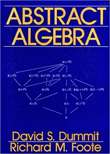
I recently wrote a series of blog posts explaining what images on the covers of math books were about, and one of these posts was an explanation of the following diagram:


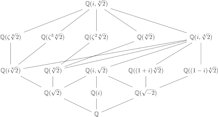
Each node in the graph is a field, and a line means the field on the higher level is an extension of the field on the lower level. For each graph like this of extension fields, there is a corresponding graph of Galois groups. Specifically, let L be the field at the top of the diagram and let E be any field in the graph.

The corresponding graph of groups replaces E with the group of group isomorphisms from L to L that leave the elements of E unchanged, the automorphisms of L that fix E. This map from fields to groups is half of a Galois connection pair. The other half is the map that takes each group to the field of elements of L fixed by G. This connection is antitone because if a field F is an extension of E, then the group of automorphisms that fix F are a subgroup of the automorphisms that fix E.

***

[1] We could think of A and B as categories, where there is a morphism between x and y iff xy. Then a monotone Galois connection between A and B is an antitone Galois connection between A and Bop.

[2] Garrett Birkhoff. Lattice Theory. American Mathematical Society Colloquium Publications, volume 25. New York, 1940.

Helmholtz resonator revisited

We finished a bottle of wine this evening, and I blew across the top as I often do. (Don’t worry: I only do this at home. If we’re ever in a restaurant together, I won’t embarrass you by blowing across the neck of an empty bottle.)

The pitch sounded lower than I expected, so I revisited some calculations I did last year.

As I wrote about here, a wine bottle is approximately a Helmhotz resonator. The geometric approximation is not very good, but the pitch prediction usually is. An ideal Helmholtz resonator is a cylinder attached to a sphere, and a typical wine bottle is more like a cylinder attached to a larger cylinder. But the formula predicting pitch is robust to departures from ideal assumptions.

As noted before, the formula for the fundamental frequency of a Helmholtz resonator is

f = \frac{v}{2\pi} \sqrt{\frac{A}{LV}}

where the variables are as follows:

  • f, frequency in Hz
  • v, velocity of sound
  • A, area of the opening
  • L, length of the neck
  • V, volume

The opening diameter was 2 cm, the neck length 9 cm, and the volume 750 cm³. All these are typical. The predicted frequency is f = 118 Hz. The measured frequency was 106 Hz, measured by the Sonic Tools phone app.

The actual frequency was about 10% lower than predicted. This is about a whole step lower in musical terms. I could certainly hear an interval that large if I heard the two pitches sequentially. But I don’t have perfect pitch, and so I’m skeptical whether I could actually notice a pitch difference of that size from memory.

Ratio test counterexample

Given a sequence a1, a2, a3, … let L be the limit of the ratio of consecutive terms:

L = \lim_{n\to\infty} \left| \frac{a_{n+1}}{a_n}\right|

Then the series

\sum_{n=1}^\infty a_n

converges if L < 1 and diverges if L > 1.

However, that’s not the full story. Here is an example from Ernesto Cesàro (1859–1906) that shows the ratio test to be more subtle than it may seem at first. Let 1 < α < β and consider the series

\frac{1}{1^\alpha} + \frac{1}{2^\beta} + \frac{1}{3^\alpha} + \frac{1}{4^\beta} + \cdots

The ratio a2n + 1 / a2n diverges, but the sum converges.

Our statement of the ratio test above is incomplete. It should say if the limit exists and equals L, then the series converges if L < 1 and diverges if L > 1. The test is inconclusive if the limit doesn’t exist, as in Cesàro’s example. It’s also inconclusive if the limit exists but equals 1.

Cesàro’s example interweaves two convergent series, one consisting of the even terms and one consisting of the odd terms. Both converge, but the series of even terms converges faster because β > α.

Related post: Cesàro summation

Whittaker and Watson

Whittaker and Watson’s analysis textbook is a true classic. My only complaint about the book is that the typesetting is poor. I said years ago that I wish someone would redo the book in LaTeX and touch it up a bit.

I found out while writing my previous post that in fact someone has done just that. That post explains the image on the cover of a reprint of the 4th edition from 1927. There’s now a fifth edition, published last year (2021).

The foreword of the fifth edition begins with this sentence:

There are few books which remain in print and in constant use for over a century; “Whittaker and Watson” belongs to this select group.

That statement is true of books in general, but it’s especially rare for math books to age so well.

The first edition came out in 1902. The book shows its age, for example, by spelling “show” with an e rather than an o. And yet I routinely run into references to the book. Nobody has written a better reference over the last century.

The new edition corrects some errors and adds references for more up-to-date results. But in some sense the mathematics in Whittaker and Watson is finished. This has a bizarre side effect: much of the material in Whittaker and Watson is no longer common knowledge precisely because the content is settled.

The kind of mathematics presented in Whittaker and Watson is very useful, but it falls between two stools. It’s too difficult for undergraduates, and it’s not a hot enough topic of research for graduate students.

When I finished my PhD, I knew some 20th century math and some 18th century math, but there was a lot of useful mathematics developed in the 19th century that I wouldn’t learn until later, the kind of math you find in Whittaker and Watson.

Someone may reasonably object that the emphasis on special functions in classical analysis is inappropriate now that we can easily compute everything numerically. But how are we able to compute things accurately and efficiently? By using libraries developed by people who know about special functions and other 19th century math! I’ve done some of this work, speeding up calculations a couple orders of magnitude on 21st century computers by exploiting arcane theorems developed in the 19th century.

Related posts

Keyhole contour integrals

The big idea

The Cauchy integral theorem says that the integral of a function around a closed path in the complex plane depends only on the poles of the integrand inside the path. You can change the path itself however you like as long as you don’t change which poles are inside. This observation is often used to compute real integrals using complex analysis.

Suppose you want to integrate a function f along (some portion of) the real line, and f extends to a function in the complex plane that is analytic except at poles. You may be able to evaluate your real integral using a complex contour, or more commonly, a limit of contours. You show that in some limit, the contribution to the integral along the parts of the contour you don’t need goes to zero, and the rest of the contour approaches the part you wanted to integrate over initially.

Keyhole contours

There area a handful of integration contours that come up most frequently, and the keyhole is one of them. The initial motivation for this post was the cover of the fourth edition of A Course of Modern Analysis by Whittaker and Watson. I’ve written a couple posts lately about the story behind images on book covers, and this is another post in that series.

E. T. Whittaker & G. N. Watson, A Course of Modern Analysis

The most recent edition has a more prosaic cover with only words and no image. However, the latest addition is much more attractive inside, having been rewritten in LaTeX.

The image on the cover is a keyhole contour. Typically the slot in the contour runs along the real axis, but the cover rotated the image 45 degrees to make it more visually appealing. The contour is used on page 118 of the fourth edition to integrate rational functions along the positive real axis [1].

Contour integration drawing

If the function you’re integrating has poles only at the locations marked by stars, then you can evaluate the integral around the contour by computing the residues of the integrand at these points. Now suppose you change the contour by making the outer circle larger, letting its radius R go to infinity, and making the inner circle shrink, letting its radius ε go to zero. If the integral along these two circular segments goes to zero in the limit, you’re left with the integral along the positive real axis.

Hankel

The keyhole contour is sometimes called the Hankel contour because Hermann Hankel used it in the 19th century to investigate special functions such as the gamma function and the eponymous Hankel functions. The first post in this series of book cover commentaries mentioned a book that has a plot of a Hankel function on the cover.

Related posts

[1] Specifically, Whittaker and Watson show how to compute the integral of xa−1 Q(x) from 0 to infinity, where Q is a rational function with no positive real zeros, and the limit of xa Q(x) is zero both as x goes to zero and as x goes to ∞.

Galois diagram

The previous post listed three posts I’d written before about images on the covers of math books. This post is about the image on the first edition of Dummit and Foote’s Abstract Algebra.

Here’s a version of the image on the cover I recreated using LaTeX.

The image on the cover appears on page 495 and represents extension fields. If you’re going through this book sequentially as a text book, it’s likely time will run out before you ever find out what the image on the cover means. If you do get to it, you get to it near the end of your course.

My diagram is topologically equivalent to the original. I took the liberty of moving things around a bit to keep the diagram from being awkwardly wide.

At the bottom of the diagram we have ℚ, the field of rational numbers. At the top of the diagram we have ℚ(i, 21/8), the smallest field containing the rational numbers, the imaginary unit i, and the eighth root of 2. Lines between fields on two levels indicate that the higher is an extension of the lower. The constant ζ in the diagram is

ζ = √i = √2(1 + i)/2.

The significance of the diagram is that extension field relationships like these are important in Galois theory. The image appears late in the book because the majority of the book is leading up to Galois theory.

Book cover posts

When a math book has an intriguing image on the cover, it’s fun to get to the point in the book where the meaning of the image is explained. I have some ideas for book covers I’d like to write about, but here I’d like to point out three such posts I’ve already written.

Weierstrass elliptic function

The book on the left is Abramowitz and Stegun, affectionately known as A&S. I believe the function plotted on the cover is the Weierstrass elliptic function, as I wrote about here.

As the image suggests, my copy of A&S has seen a bit of wear. At one point the cover fell off and I put it back on with packing tape.

Möbius transformation of circles

The book in the middle is my well-worn copy of my undergraduate complex analysis text. The cover is a bit dirty and pages are falling out, a sort of Velveteen rabbit of math books.

I haven’t written a post about the cover per se, but I did write about the necessary math to recreate the image on the cover here. That post explains how to compute the image of a circle under a Möbius transformation. The image on the left is mapped to the image on the right via the function

f(z) = 1/(z − α).

Here α is the point on the right where all the outer circles are tangent. If you wanted to reconstruct the image on the cover, it would be easier to proceed from right to left: start with the image on the right because it’s easier to describe, and apply the inverse transformation using the instructions in the blog post to produce the image on the left.

Hankel functions

I wrote about the book on the right here. I believe the image on the cover is the plot of a Hankel function.

Updates

Here’s a post explaining the image on the cover Abstract Algebra by Dummit and Foote.

And here is a post explaining the image on the cover of A Course of Modern Analysis by Whittaker and Watson.


Aristeia

When I had a long commute, I listened to everything I could get my hands on. That included a lot of Teaching Company courses from my local library. A couple of the courses I listened to were Elizabeth Vandiver lecturing on classics.

One of the things I remember her talking about was aristeia, a character’s moment of greatest glory, often shortly before they die.

That was years ago, but I remembered it recently when I was watching the final episode of the current season of Stranger Things. Eddie Munson gives what he had said would be “the most metal concert in the history of the world.” It is by far his greatest hour.

I would say “spoiler alert” about what happens next, but Elizabeth Vandiver gave the spoiler long before Stranger Things was written.

Eddie Munson playing Master of Puppets in Stranger Things

Gaussian elimination

Carl Friedrich Gauss

When you solve systems of linear equations, you probably use Gaussian elimination, even if you don’t call it that. You may learn Gaussian elimination before you see it formalized in terms of matrices.

So if you’ve had a course in linear algebra, and you sign up for a course in numerical linear algebra, it’s natural to expect that Gaussian elimination would be one of the first things you talk about. That was my experience, and it was painful. I had this odd mixture of feeling like I already knew what the professor was talking about, while at the same time feeling lost.

Trefethen and Bau do not start their numerical linear algebra textbook with Gaussian elimination, and they explain why in the preface:

We have departed from the customary practice by not starting with Gaussian elimination. That algorithm is atypical of numerical linear algebra, exceptionally difficult to analyze, yet at the same time tediously familiar to every student in a course like this. Instead, we begin with the QR factorization, which is more important, less complicated, and fresher idea to most students.

It’s reassuring to hear experts in numerical linear algebra admit that Gaussian elimination is “exceptionally difficult to analyze.” The algorithm is not exceptionally difficult to perform; children learn to manually execute the algorithm. But it is surprisingly difficult, and tedious, to analyze.

Numerical analysts like Trefethen and Bau have much more sophisticated questions in mind than how you would naively carry out the algorithm by hand. Numerical analysts are concerned, for example, with stability.

If your coefficients are known exactly and you carry out your arithmetic exactly, then you get an exact result. But can a small change to your inputs, say due to measurement uncertainty, or the inevitable loss of precision from floating point arithmetic, make a large change in your results? Absolutely, unless you use pivoting. But with pivoting, Gaussian elimination is stable [1].

After taking an introductory linear algebra course, you know how to solve any linear system of equations in principle. But when you actually want to compute the solution accurately, efficiently, at scale, in a real computer, with real data, things can get much more interesting. Many people have devoted their careers to doing in practice what high school students know how to do in principle.

Related posts

[1] There are matrices for which Gaussian elimination is unstable, but they are rare. It’s been shown that they are rare in the sense of having low probability, but more importantly they never arise naturally in applied problems.