Major League Baseball and number theory

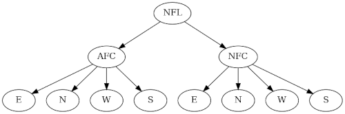
The previous post took a mathematical look at the National Football League. This post will do the same for Major League Baseball.

Like the NFL, MLB teams are organized into a nice tree structure, though the MLB tree is a little more complicated. There are 32 NFL teams organized into a complete binary tree, with a couple levels collapsed. There are 30 MLB teams, so the tree structure has to be a bit different.

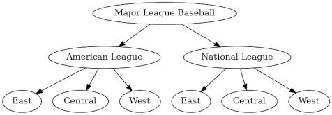
MLB has leagues rather than conferences, but the top-level division is into American and Nation as with the NFL. So the top division is into the American League and the National League.

And as with football, the next level of the hierarchy is divisions. But baseball has three divisions—East, Central, and West—in contrast to four in football.

Each division has five baseball teams, while each football division has four teams.

Here’s the basic tree structure.

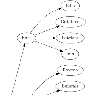
Under each division are five teams. Here’s a PDF with the full graph including teams.

Geography

How do the division names correspond to actual geography?

Within each league, the Central teams are to the west of the East teams and to the east of the West teams, with one exception: in the National League, the Pittsburgh Pirates are a Central division team, but they are east of the Atlanta Braves and Miami Marlins in the East division. But essentially the East, Central, and West divisions do correspond to geographic east, center, and west, within a league.

Numbering

We can’t number baseball teams as elegantly as the previous post numbered football teams. We’d need a mixed-base number. The leading digit would be binary, the next digit base 3, and the final digit base 5.

We could number the teams so that you could tell the league and division of the team by looking at the remainders when the number is divided by 2 and 3, and each team is unique mod 5. By the Chinese Remainder Theorem, we can solve the system of congruence equations mod 30 that specify the value of a number mod 2, mod 3, and mod 5.

If we number the teams as follows, then even numbered teams are in the American League and odd numbered teams are in the National League. When the numbers are divided by 3, those with remainder 0 are in an Eastern division, those with remainder 1 are in a Central division, and those with remainder 2 are in a Western division. Teams within the same league and division have unique remainders by 5.

  1. Cincinnati Reds
  2. Oakland Athletics
  3. Philadelphia Phillies
  4. Minnesota Twins
  5. Arizona Diamondbacks
  6. Boston Red Sox
  7. Milwaukee Brewers
  8. Seattle Mariners
  9. Washington Nationals
  10. Chicago Whitesocks
  11. Colorado Rockies
  12. New York Yankees
  13. Pittsburgh Pirates
  14. Texas Rangers
  15. Atlanta Braves
  16. Cleveland Guardians
  17. Los Angeles Dodgers
  18. Tampa Bay Rays
  19. St. Louis Cardinals
  20. Houston Astros
  21. Miami Marlins
  22. Detroit Tigers
  23. San Diego Padres
  24. Toronto Blue Jays
  25. Chicago Cubs
  26. Los Angeles Angels
  27. New York Mets
  28. Kansas City Royals
  29. San Francisco Giants
  30. Baltimore Orioles

Related posts

A mathematical look at the NFL

This post will look at the National Football League through the lens of graph theory, topology, and binary numbers.

The NFL has a very nice tree structure, which isn’t too surprising in light of the need to make tournament brackets. The NFL is divided into two conferences, the American Football Conference and the National Football Conference.

Tree structure

Each conference is divided into four divisions named after geographical regions. Since this is a mathematical post, I’ve listed the regions counterclockwise starting in the east because that’s how mathematicians do things.

NFL -> AFC<br /> NFL -> NFC<br /> AFC -> AFCE<br /> AFC -> AFCN<br /> AFC -> AFCW<br /> AFC -> AFCS<br /> NFC -> NFCE<br /> NFC -> NFCN<br /> NFC -> NFCW<br /> NFC -> NFCS

Each division has four teams. Adding each team under its division would make an awkwardly wide graph. I made a graph of the entire tree, rotated so that image is long rather than wide. Here’s a little piece of it.

The full image is available here.

Geography

Now you may wonder how well the geographic division names correspond to geography. For example, the Dallas Cowboys are in the NFC East, and it’s a little jarring to hear Texas called “east.”

But within each conference, all the “East” teams are indeed east of all the West teams. And with one exception, all the North teams are indeed north of the South teams. The Indianapolis Colts are the exception. The Colts are in the AFC South, but are located to the north of the Cincinnati Bengals and the Baltimore Ravens in the AFC North.

This geographical sorting only applies within a conference. The Dallas Cowboys, for example are east of all the West teams within their conference, but they are west of the Kansas City Chiefs in the AFC West.

Here’s where topology comes in: you can make the division names match their geography if you morph the map of the United States pulling Indianapolis south of its geometric location.

Binary numbers

The graph structure of the NFL is essentially a full binary tree; you could make it into a binary tree by introducing a sub-conference layer and grouping the teams into pairs.

You could number the NFL teams with five bits: one for the conference, two for the division, and two more for the team. We could make the leading bit 0 for the AFC and 1 for the NFC. Then within each division, we could use 00 for East, 01 for North, 10 for West, and 11 for South. As mentioned above, this follows the mathematical convention of angles increasing counterclockwise starting at the positive x-axis.

The table above is an SVG image; here is the same data in plain text.

Related posts

How Mr. Benjamin squares numbers

This post is a sequel to the post How Mr. Bidder calculated logarithms published a few days ago. As with that post, this post is based on an excerpt from The Great Mental Calculators by Steven B. Smith.

Smith’s book says Arthur Benjamin squares large numbers using the formula

n² = (n + a)(na) + a²

where a is chosen to make the multiplication easier, i.e. to make n + a or na a round number. The method is then applied recursively to compute a², and the process terminates when you get to a square you have memorized. There are nuances to using this method in practice, but that’s the core idea.

The Great Mental Calculators was written in 1983 when Benjamin was still a student. He is now a mathematics professor, working in combinatorics, and is also well known as a mathemagician.

Major system

Smith quotes Benjamin giving an example of how he would square 4273. Along the way he needs to remember 184 as an intermediate result. He says

The way I remember it is by converting 184 to the word ‘dover’ using the phonetic code.

I found this interesting because I had not heard of anyone using the Major system (“the phonetic code”) in real time. This system is commonly used to commit numbers to long-term memory, but you’d need to be very fluent in the system to encode and decode a number in the middle of a calculation.

Maybe a lot of mental calculators use the Major system, or some variation on it, during calculations. Most calculators are not as candid as Benjamin in explaining how they think.

Related posts

Bounding derivatives of the sinc function

The sinc function is defined either as sin(x)/x or as sin(πx)/πx. We’ll use the former definition here because we’ll cite a paper that uses that definition.

Here’s a plot of the sinc function and its first two derivatives.

Thomas Grönwall proposed a problem to the American Mathematical Monthly in 1913 [1] bounding the derivatives of the sinc function:

\left| \frac{d^n}{dx^n} \frac{\sin x}{x}\right| \leq \frac{1}{n+1}

Seven years later, Dunkel gave an elegant proof. Perhaps Grönwall had a proof and was proposing his inequality as a challenge, or maybe it was a conjecture at the time he published it. In any case, the proof by Dunkel is very nice. He sets

y = sin(x)/x

and repeatedly differentiates both sides of the equation

xy = sin(x).

See the details in Dunkel’s solution.

I don’t know of an application of Grönwall’s inequality offhand. But the sinc function is common in signal processing, and so maybe his inequality has applications there.

(By “Grönwall’s inequality” I mean the inequality above. There is another theorem also known as Grönwall’s inequality that is commonly applied in differential equations.)

[1] Gronwall, T. H. (1913). Problem 339. Amer. Math. Monthly. 20: 196.

[2] Dunkel, O., (1920). Solution to Problem 339. Amer. Math. Monthly. 27: 81–85.

Another Napoleon-like theorem

A little while back I wrote about Napoleon’s theorem for triangles. A little later I wrote about Van Aubel’s theorem, a sort of analogous theorem quadrilaterals. This post presents another analog of Napoleon’s theorem for quadrilaterals.

Napoleaon’s theorem says that if you start with any triangle, and attach equilateral triangles to each side, the centroids of these new triangles are the vertices of an equilateral triangle.

So if you attach squares to the sides of a quadrilateral, are their centroids the vertices of a square? In general no.

But you can attach squares to two sides, and special rectangles to the other two sides, and the centroids will form the corners of a square. Specifically, we have the following theorem by Stephan Berendonk [1].

If you erect squares on the two “nonparallel” sides of a trapezoid and a rectangle on each of the two parallel sides, such that its “height” is equal to the length of the opposite side of the trapezoid, then the centers of the four erected quadrangles will form the vertices of a square.

Here’s an illustration. Berendonk’s theorem asserts that the red quadrilateral is a square.

[1] Stephan Berendonk. A Napoleonic Theorem for Trapezoids. The American Mathematical Monthly, April 2019, Vol. 126, No. 4, pp. 367–369

Playfair cipher

The Playfair cipher was the first encryption technique to encrypt text two letters at a time. Instead of substituting one letter for another, it substitutes one pair of letters for another pair. This makes the method more secure than a simple substitution cipher, but hardly secure by modern standards.

The Playfair cipher was used (and broken) during the first world war. I vaguely remember reading somewhere that the cipher took about an hour to break using pencil and paper. It was secure in the sense that it could be used for messages that only needed to be secure for less time than it took to break the method. It was more secure than simple substitution, and easy to encrypt and decrypt manually.

True to Stigler’s law of eponymy, the Playfair cipher was not named after its inventor, Charles Wheatstone of Wheatstone bridge fame, but after Lyon Playfair who popularized the method. Playfair acknowledged Wheatstone, but his name stuck to the method nevertheless.

Message preparation

The Playfair cipher uses a 5 × 5 grid of letters, so some letter of the Roman alphabet has to go. A common choice was to use the same letter for I and J. (A variation on the method using a 6 × 6 grid of letters and digits would not have to leave out any letters.)

For reasons that will soon be apparent, double letters had to be broken up, say with an X. So “FOOTBALL” would become “FOXOTBALXL.” Amusingly, “MISSISSIPPI” would become “MISXSISXSIPXPI.”

After eliminating Js and splitting double letters, the message is divided into pairs. So FOXOTBALXL becomes FO XO TB AL XL.

Encryption algorithm

The key for the encryption method is the arrangement of the letters in a square. In practice, the key would be some word or phrase that was used to permute the alphabet, and then that permutation was filled into the grid.

Here’s a grid I constructed by asking Python for a random permutation of the alphabet.

IFTVX PCGDY RNHQK EBSLA OUMWZ

Given a pair of letters, the two letters either lie on the same row, the same column, or are in different rows and columns. (This is why you break up double letters.)

If the two letters lie in the same row, advance each letter one position, wrapping around if necessary. For example, IT would be encrypted as FV, and TX would be encrypted as VI.

If two letter line in the same column, proceed analogously, moving each letter down. So TH would be encrypted as GB and OI would be encrypted as IP.

Finally, if the two letters are in different rows and columns, they form the diagonal corners of a rectangle. Replace the two letters with the letters on the remaining corners. For example, IH becomes TR, HE becomes RB, GW becomes DM, etc.

Cryptanalysis

Just as you can attack a simple substitution cipher by looking at letter frequencies, you can attack a Playfair cipher by looking at bigram frequencies. You can find these frequencies for English text on Peter Norvig’s site. TH sticks out in bigram frequencies similarly to how E sticks out in letter frequencies. However, bigram frequencies are more evenly distributed than letter frequencies.

As I pointed out in the previous post, making a mapping between 676 pairs of letters to a randomly generated list of 676 other pairs of letters will not create a secure cipher. But Playfair is much weaker than such a random assignment. There is a lot of structure to the Playfair cipher. This makes it more convenient to use, and easier to break.

Suppose pairs of letters where mapped to random pairs of letters and you learn that GB is the encrypted form of TH. What have you learned about decrypting any other pair? Nothing, except that you’ve eliminated 1 out of 676 possibilities.

But if you learn that a Playfair cipher sends TH to GB, you learn that either (1) T, H. G, and B all lie in the same row or column, or (2) that T and B are in the same column, G and B are in the same column, T and G are in the same row, and H and B are in the same row.

Symmetry

If we rotate the rows or columns in our encryption matrix, nothing changes. This is easy to see in the case when two letters are in the same row or in the same column. It’s a little harder to see but still true when the letters are in different rows and columns.

For example, consider the following encryption matrix, formed by rotating the columns two positions and the rows one position.

GDYPC
HQKRN
BLAES
MWZOU
TVXIF

If you work through all the examples above, you’ll see that they remain the same. IT still goes to FV etc.

The reason rotating columns or rows doesn’t make a difference is that in matrix notation, the encryption algorithm does not depend on the subscripts per se but the difference in subscripts mod 5.

It almost doesn’t matter if you transpose the encryption matrix. If you transpose a matrix, elements that were in the same row are now in the same column and vice versa. When two letters are not in the same row or column, transposing the encryption matrix transposes the encrypted pair. In the example above HE goes to RB. If we transpose the encryption matrix, HE goes to BR.

We said above that the key to a Playfair cipher is a permutation of the alphabet. But many keys correspond to the same encryption mapping. The analyst doesn’t need to recover the original encryption matrix but only some rearrangement of it.

Related posts

Simple substitution ciphers over a gargantuan alphabet

Simple substitution ciphers replace one letter with another. Maybe A goes to W, B goes to G, C goes to A, etc.

These ciphers are famously easy to break, so easy that they’re common in puzzle books. Here’s one I made [1] for this post in case you’d like to try it.

X RF SXIIXKW XK IYZ UXINYZK HT IYZ CXIICZ YHJSZ RI FZGTXZCG, HJQ SZNHKG TRQF BYXNY XS NJI HTT EV IYZ QXGWZ RKG R MJRQIZQ-FXCZ RNQHSS IYZ TXZCGS TQHF HJQ YHFZ LCRNZ, BYZQZ VHJ RQZ. X RF BQXIXKW R EHHU. XK XI X RF SLZRUXKW IH VHJ. EJI X RF RCSH SLZRUXKW IH IYZ BHQCG. IH EHIY X HBZ RK RNNHJKIXKW.

As is common in puzzle books, I kept the spaces and punctuation.

When you learn that simple substitution is breakable, you might reasonably think that the problem is the small alphabet size. What if you replaced pairs of letters with pairs of letters, effectively working over an alphabet of size 26² = 676. That’s an improvement, but it’s still not secure. It could be broken manually in a few hours, depending on the length of the text, and of course could be broken quickly using a computer.

If we want a cipher to be secure against computer-aided cryptanalysis, we’re going to need a much bigger alphabet.

The Roman alphabet has 26 letters, which can be expressed in 5 bits. Pairs of Roman letters would require 10 bits. What if we used a 32-bit alphabet, substituting 32-bit sequences with other 32-bit sequences? This is working over an alphabet of over 4 billion symbols. Surely that’s secure? Nope.

What if we use blocks of 128 bits? This is working over an alphabet of size

2128 = 340,282,366,920,938,463,463,374,607,431,768,211,456.

Nope. Still not good enough. Because you can see the penguin.

Original encrypted Tux image

The image above is a famous example of a downfall of simple substitution, albeit over a gargantuan alphabet. The image was created by taking a graphic of the Linux mascot and encrypting the bits using 128-bit encryption. Each block of 128 bits goes to a unique, essentially random replacement. Each block is well encrypted. But there are repetitive blocks in the original that become repetitive blocks in the encrypted version.

The AES (Rijndael) encryption algorithm is a good algorithm, but in the example above it was used poorly. It was used in electronic code book mode (ECB), something that nobody would do in practice.

In practice, you might do something like cipher block chaining where you XOR each block with the encrypted version of the previous block. You could think of this as a clever way of using a simple substitution over an enormous alphabet. You look up the substitution of each block, but then XOR its bits with the previously encrypted block. Now repetitive input does not produce repetitive output. You cannot see the penguin. The penguin image becomes random-looking static.

Related posts

[1] I produced the cryptogram using

    cat myfile | tr [a-z] [A-Z] | tr [A-Z] ...

where “…” is a permutation of the 26 upper case letters.

How Mr. Bidder calculated logarithms

George Parker Bidder (1806–1878) was a calculating prodigy. One of his feats was mentally calculating logarithms to eight decimal places. This post will explain his approach.

I’ll use “log” when the base of the logarithm doesn’t matter, and add a subscript when it’s necessary to specify the base. Bidder was only concerned with logarithms base 10.

Smooth numbers

If you wanted to calculate logarithms, a fairly obvious strategy would be to memorize the logarithms of small prime numbers. Then you could calculate the logarithm of a large integer by adding the logarithms of its factors. And this was indeed Bidder’s approach. And since he was calculating logarithms base 10, so he could make any number into a integer by shifting the decimal and then subtracting off the number of places he moved the decimal after taking the log of the integer.

Numbers with only small prime factors are called “smooth.” The meaning of “small” depends on context, but we’ll say numbers are smooth if all the prime divisors are less than 100. Bidder knew the logs of all numbers less than 100 and the logs of some larger numbers.

Rough numbers

But what to do with numbers that have a large prime factor? In this case he used the equation

log(a + b) = log(a(1 + b/a)) = log(a) + log(1 + b/a).

So if a number n doesn’t factor into small primes, but it is close to a number a that does factor into small primes, you’re left with the problem of finding log(1 + b/a) where b = na and the fraction b/a is small.

At this point you may be thinking that now you could use the fact that

log(1 + x) ≈ x

for small x. However, Bidder was interested in logarithms base 10, and the equation above is only valid for natural logarithms, logarithms base e. It is true that

loge(1 + x) ≈ x

but

log10(1 + x) ≈ log10(e) x = 0.43429448 x.

Bidder could have used 0.43429448 x as his approximation, but instead he apparently [1] used a similar approximation, namely

log(1 + b/a) ≈ log(1 + 10m) 10m b/a

where b/a is between 10m−1 and 10m. This approximation is valid for logarithms with any base, though Bidder was interested in logs base 10 and had memorized log101.01, log101.001, log101.0001, etc. [2]

Finding nearby smooth numbers

To get eight significant figures, the fraction b/a must be on the order of 0.001 or less. But not every number n whose log Bidder might want to calculate is so close to a smooth number. In that case Bidder might multiply n by a constant k to find a number so that kn is close to a smooth number, take the log of kn, then subtract log k.

Smith says in [1] “For example, to obtain log 877, he would multiply 877 by 13, which gives 11,401, or 600 × 19 + 1.” Then he could calculate

log(877) = log(13*877) −- log(13) = log(11400) + log(1/11400) − log(13)

and use his algorithm for approximating log(1/11400).

I can’t imagine thinking “Hmm. 877 isn’t close enough to a smooth number, but if I multiply it by 13 it will be.” But apparently Bidder thought that way.

Related posts

Here is a simple way to approximate logarithms to a couple significant figures without having to memorize anything.

See also this post on mentally calculating other functions to similar accuracy.

Notes

[1] This equation comes from The Great Mental Calculators by Steven B. Smith. Bidders methods are not entirely known, and Smith prefaces the approximation above by saying “it appears that Bidder’s approximation was …”.

[2]

|-------+-------------|
|     x | log_10(1+x) |
|-------+-------------|
| 10^-2 |  0.00432137 |
| 10^-3 |  0.00043408 |
| 10^-4 |  0.00004342 |
| 10^-5 |  0.00000434 |
| 10^-6 |  0.00000043 |
| 10^-7 |  0.00000004 |
|------+--------------|

Sines of integers

The sine function has period 2π, an irrational number. and so if we take the sines of the integers, we’re going to get a somewhat random sequence. (I’m assuming, as always that we’re working in radians. The sines of integer numbers of degrees are much less interesting.)

Here’s a plot of the sines of 0, 1, 2, …, 99.

The points are not literally random, but they’re what Marsaglia would call higgledy-piggledy [1].

Since the points are higgledy-piggledy, it doesn’t seem possible that we could find a lower bound on |sin(n)|, but there is one. For all positive integers n,

|sin(n)| > 2n.

This result may be due to Christopher Stuart, but in any case he proved [2] a stronger version of this theorem, showing that the 2 on the right hand side can be replaced with any number

α > (sin(3))−1/3 = 1.9207….

Related posts

[1] “If the numbers are not random, they are at least higgledy-piggledy.” — RNG researcher George Marsaglia

[2] Christopher Stuart. An Inequality Involving sin(n). The American Mathematical Monthly , Feb 2018, Vol. 125, No. 2, pp. 173–174

Derive or memorize?

A lot of smart people have a rule not to memorize anything that they can derive on the spot. That’s a good rule, up to a point. But past that point it becomes a liability.

Most students err on the side of memorizing too much. For example, it’s common for students to memorize three versions of Ohms law:

  • V = IR
  • I = V/R
  • R = V/I.

Not only is this wasteful, tripling the number of facts to remember, it’s also error prone. When you memorize things without understanding them, you have no way to detect mistakes. Someone memorizing the list above might think “Is I = V/R or R/V?” but someone who knows what the terms mean will know that more resistance means less current, so the latter cannot be right.

I got through my first probability class in college without memorizing anything. I worked every problem from first principles, and that was OK. But later on I realized that even though I could derive things from scratch every time I needed them, doing so was slowing me down and keeping me from seeing larger patterns.

The probability example stands out in my mind because it was a conscious decision. I must have implicitly decided to remember things in other classes, but it wasn’t such a deliberate choice.

I’d say “Don’t memorize, derive” is a good rule of thumb. But once you start to say to yourself “Here we go again. I know I can derive this. I’ve done it a dozen times.” then maybe it’s time to memorize the result. To put it another way, don’t memorize to avoid understanding. Memorize after thoroughly understanding.

Related post: Just-in-case versus just-in-time