Relativistic multiplication

A couple years ago I wrote about relativistic addition. Given two numbers in the interval (-c, c) you can define their relativistic sum by

x \oplus y \equiv \frac{x + y}{1 + \dfrac{xy}{c^2}}

We can set c = 1 without loss of generality.

Given this exotic definition of addition, what is multiplication?

We’d expect 2 ⊙ x to be the same as xx, and 3 ⊙ x to be the same as xxx, etc. If you stare at these examples you may come up with the proposal

n \odot x = \frac{(1+x)^n-(1-x)^n}{(1-x)^n+(1+x)^n}

It turns out this works for all positive integers n. We can replace n with any real number r and take this as the definition of multiplication by any real number. (Because x is between -1 and 1, the terms in parentheses are always positive and so there’s no difficulty defining real exponents.)

Now what kind of algebraic properties does this multiplication have? It’s not symmetric. The left argument of ⊙ can be any real number, while the right argument has to be in (-1, 1). And if the first argument r happens to be in (-1, 1), it’s not generally the case that rx equals xr.

What we have is scalar multiplication in a vector space. If we define vectors to be numbers in the interval (-1, 1), with vector addition defined by ⊕, and scalar multiplication defined by ⊙, all the axioms of a vector space are satisfied.

Reference: Michael A. Carchidi. Generating Exotic-Looking Vector Spaces. The College Mathematics Journal, Vol. 29, No. 4, pp. 304–308

Circulant matrices, eigenvectors, and the FFT

A circulant matrix is a square matrix in which each row is a rotation of the previous row. This post will illustrate a connection between circulant matrices and the FFT (Fast Fourier Transform).

Circulant matrices

Color in the first row however you want. Then move the last element to the front to make the next row. Repeat this process until the matrix is full.

The NumPy function roll will do this rotation for us. Its first argument is the row to rotate, and the second argument is the number of rotations to do. So the following Python code generates a random circulant matrix of size N.

    import numpy as np

    np.random.seed(20230512)
    N = 5
    row = np.random.random(N)
    M = np.array([np.roll(row, i) for i in range(N)])

Here’s the matrix M with entries truncated to 3 decimal places to make it easier to read.

    [[0.556 0.440 0.083 0.460 0.909]
     [0.909 0.556 0.440 0.083 0.460]
     [0.460 0.909 0.556 0.440 0.083]
     [0.083 0.460 0.909 0.556 0.440]
     [0.440 0.083 0.460 0.909 0.556]]    

Fast Fourier Transform

The Fast Fourier Transform is a linear transformation and so it can be represented by a matrix [1]. This the N by N matrix whose (j, k) entry is ωjk where ω = exp(-2πi/N), with j and k running from 0 to N – 1. [2]

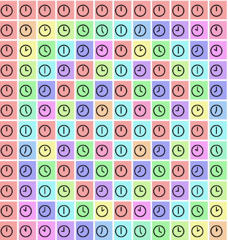
Each element of the FFT matrix corresponds to a rotation, so you could visualize the matrix using clocks in each entry or by a cycle of colors. A few years ago I created a visualization using both clock faces and colors:

Eigenvectors and Python code

Here’s a surprising property of circulant matrices: the eigenvectors of a circulant matrix depend only on the size of the matrix, not on the elements of the matrix. Furthermore, these eigenvectors are the columns of the FFT matrix. The eigenvalues depend on the matrix entries, but the eigenvectors do not.

Said another way, when you multiply a circulant matrix by a column of the FFT matrix of the same size, this column will be stretched but not rotated. The amount of stretching depends on the particular circulant matrix.

Here is Python code to illustrate this.

    for i in range(N):
        ω = np.exp(-2j*np.pi/N)
        col1 = np.array([ω**(i*j) for j in range(N)])
        col2 = np.matmul(M, col1)
        print(col1/col2)

In this code col1 is a column of the FFT matrix, and col2 is the image of the column when multiplied by the circulant matrix M. The print statement shows that the ratios of each elements are the same in each position. This ratio is the eigenvalue associated with each eigenvector. If you were to generate a new random circulant matrix, the ratios would change, but the input and output vectors would still be proportional.

Notes

[1] Technically this is the discrete Fourier transform (DFT). The FFT is an algorithm for computing the DFT. Because the DFT is always computed using the FFT, the transformation itself is usually referred to as the FFT.

[2] Conventions vary, so you may see the FFT matrix written differently.

Packing versus unpacking

I usually think of an instructor as someone who unpacks things, such as unpacking the meaning of an obscure word or explaining a difficult concept.

Last night I was trying to read some unbearably dry medical/legal material and thought about how an instructor might also pack things, wrapping dry material in some sort of story or illustration to make it more palatable.

I’ve often thought it would be nice to have someone explain this or that. I hadn’t really thought before that it would be nice to have someone make perfectly clear material more bearable to absorb, but I suppose that’s what a lot of instructors do. I was able to avoid courses that needed such an instructor, for which I am grateful, but I could imagine how a good instructor might make a memorization-based course tolerable.

How faithful can a map be?

It’s well known that you cannot map a sphere onto the plane without distortion. You can’t map the entire sphere to the plane at all because a sphere and a plane are not topologically equivalent.

But even if you want to map a relatively small portion of globe to paper, say France, with about 0.1% of the globe’s area, you’ll have to live with some distortion. How can we quantify this distortion? How small can it be?

We know the result has to vary with area. We expect it to approach zero as area on the globe goes to zero: the world is not flat, but it is locally flat. And we expect the amount of distortion to go to infinity as we take in more of the globe’s area. We expect to be able to make a map of France without too much distortion, less distortion than making a map of Australia, but more distortion than making a map of Lichtenstein.

This problem was solved a long time ago, and John Milnor wrote an expository article about it in 1969 [1].

Defining distortion

The way to quantify map distortion is to look at the ratio of distances on the globe to distances on paper. We measure the distance between points on the globe by geodesic distance, the length of the shortest path between two points. We’d like the ratio of distances on a globe to distances on a map to be constant, but this isn’t possible. So we look at the minimum and maximum of this ratio. In a good map these two ratios are roughly the same.

Milnor uses

dS(x, y)

to denote the distance between two points x and y on a sphere, and

dE(f(x), f(y))

for the distance between their image under a projection to the Euclidean plane.

The scale of a map with respect to points x and y is the ratio

dE(f(x), f(y)) / dS(x, y).

Let σ1 be the minimum scale as x and y vary and let σ2 be the maximum scale. The distortion of the projection f is defined to be

δ = log(σ21).

When σ1 and σ2 are approximately equal, δ is near 0.

Example: Mercator projection

One feature of the Mercator projection is that there is no distortion along lines of constant latitude. Given two points on the equator (less than 180° apart) their distance on a Mercator projection map is strictly proportional to their distance on the globe. The same is true for two points on the flat part of the US-Canada border along the 49th parallel, or two points along the 38th parallel dividing North Korea and South Korea.

For points along a parallel (i.e. a line of latitude) the scale is constant, such as a thousand miles on the globe corresponding to an inch on the map. We have σ1 = σ2 and so δ = 0.

The distortion in the Mercator projection is all in the vertical direction; distances along a meridian are distorted. Mercator maps latitude φ to something proportional to

φ ↦ log( sec φ + tan φ ).

Near the equator sec φ ≈ 1, tan φ ≈ φ, and the image of φ is approximately φ. But as φ approaches 90° the secant and tangent terms become unbounded and the distortion goes to infinity. You could use the equation for the Mercator projection of latitude to calculate the distortion of a “rectangle on a globe.”

Minimizing distortion

Let Dα be a disk geodesic radius α radians where 0 < α < π. Then Milnor shows that the minimum possible distortion when mapping Dα to the plane is

δ0 = log(α / sin α).

This map is realizable, and is unique up to similarity transformations of the plane. It is known in cartography as the azimuthal equidistant projection.

For small values of α the distortion is approximately α²/6, or 2/3 of the ratio of the area of Dα to the area of the globe.

We said earlier that France takes up about 0.1% of the earth’s surface, and so the minimum distortion for a map of France would be on the order of 0.0007.

[1] John Milnor. A Problem in Cartography. American Mathematical Monthly, December 1969, pp. 1102–1112.

Recognizing three-digit primes

If a three-digit number looks like it might be prime, there’s about a 2 in 3 chance that it is.

To be more precise about what it means for a number to “look like a prime,” let’s say that a number is obviously composite if it is divisible by 2, 3, 5, or 11. Then the following Python code quantifies the claim above.

    from sympy import gcd, isprime

    obviously_composite = lambda n: gcd(n, 2*3*5*11) > 1

    primes = 0
    nonobvious = 0

    for n in range(100, 1000):
        if not obviously_composite(n):
            nonobvious += 1
            if isprime(n):
                primes += 1
    print(primes, nonobvious)

This shows that out of 218 numbers that are not obviously composite, 143 are prime.

This is a fairly conservative estimate. It doesn’t consider 707 an obvious composite, for example, even though it’s pretty clear that 707 is divisible by 7. And if you recognize squares like 169, you can add a few more numbers to your list of obviously composite numbers.

Expected distance between points in a cube

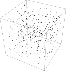
random samples from a cube

Suppose you randomly sample points from a unit cube. How far apart are pairs of points on average?

My intuition would say that the expected distance either has a simple closed form or no closed form at all. To my surprise, the result is somewhere in between: a complicated closed form.

Computing the expected value by simulation is straight forward. I’ll make the code a little less straight forward but more interesting and more compact by leveraging a couple features of NumPy.

    import numpy as np

    dimension = 3
    reps = 10000

    cube1 = np.random.random((reps, dimension))
    cube2 = np.random.random((reps, dimension))
    distances = np.linalg.norm(cube1 - cube2, axis=1)
    print(distances.mean())

This gives a value of 0.6629. This value is probably correct to two decimal places since the Central Limit Theorem says our error should be on the order of one over the square root of the number of reps.

In fact, the expected value given here is

\frac{4}{105} + \frac{17}{105}\sqrt{2} - \frac{2}{35}\sqrt{3} + \frac{1}{5}\log(1 + \sqrt{2}) + \frac{2}{5}\log(2 + \sqrt{3}) - \frac{1}{15}\pi

which evaluates numerically to 0.661707….

The expression for the expected value is simpler in lower dimensions; it’s just 1/3 in one dimension. In higher dimensions there is no closed form in terms of elementary functions and integers.

Incidentally, the image above was made using the following Mathematica code.

    pts = RandomPoint[Cube[], 10^3];
    Graphics3D[{PointSize[Small], Point[pts], Opacity[0.3]}, Boxed -> True]

Sine of factorial degrees

I was looking back at a post about the Soviet license plate game and was reminded of the amusing identity

sin (n!)° = 0

for n ≥ 6. Would it be possible to find sin (n!)° in closed form for all positive integers n?

For this post I’ll make an exception to my usual rule and assume all angles are in degrees.

First of all, sin 5! = √3/2 so we’re off to a good start.

Next, let’s look at sin 4!. If we ask Mathematica, we get nowhere. Entering

    Sin[24 Degree]

returns Sin[24°]. I tried a few Simplify and Expand commands but couldn’t coax Mathematica into revealing a closed form.

It would seem we’re stuck, but we’re not. For reasons given here we can find sin 3:

\sin 3^\circ = \frac{1}{4} \sqrt{8 - \sqrt{10 - 2 \sqrt{5}} - \sqrt{3} \left(1 + \sqrt{5}\right)}

And if we can find sin 3, we can use a double angle identity to get sin 6, sin 12, and sin 24.

So we can compute sin n! for n ≥ 3. But we really are stuck at this point. The sine of 1 degree or 2 degrees cannot be computed in closed form [1]. However, there are clever ways to numerically compute these values that go back to Medieval astronomers.

We can find sine of 6, 12, and 24 in closed form, so let’s actually do it.

    sin3 =  Sqrt[8 - Sqrt[10 - 2 Sqrt[5]] - Sqrt[3] (1 + Sqrt[5])]/4
    sin6 = 2 sin3 Sqrt[1 - sin3^2]
    sin12 = 2 sin6 Sqrt[1 - sin6^2]
    sin24 = 2 sin12 Sqrt[1 - sin12^2]

We can apply Simplify to clean up these expressions. The sine of 12 degrees cleans up nicely, though the others are still complicated after asking Mathematica for a simplification.

\begin{align*} \sin 6^\circ &= \frac{1}{4 \sqrt{-\frac{2}{\sqrt{30-6 \sqrt{5}}+\sqrt{30 \left(5-\sqrt{5}\right)}+2 \left(\sqrt{5}-9\right)}}} \\ \sin 12^\circ &= \frac{1}{4} \sqrt{7-\sqrt{5}-\sqrt{30-6 \sqrt{5}}} \\ \sin 24^\circ &= \frac{1}{4 \sqrt{-\frac{2}{\sqrt{30-6 \sqrt{5}}+\sqrt{30 \left(5-\sqrt{5}\right)}-2 \left(7+\sqrt{5}\right)}}} \end{align*}

[1] Depending on what you mean by “closed form.” I believe the sine of 1 degree can be written in terms of radicals, but the expression involves imaginary numbers that cannot be removed, even though the expression results in a real number.

Update: See the comments for a link to a paper confirming the footnote above and giving complex expressions for the sine of one degree.

LTI operators commute

Here’s a simple but surprising theorem from digital signal processing: linear, time-invariant (LTI) operators commute. The order in which you apply LTI operators does not matter.

Linear in DSP means just you’d expect from seeing linear defined anywhere else: An operator L is linear if given any two signals x1 and x2, and any two constants α and β,

Lx1 + βx2) = αL(x1) + βL(x2).

Time-invariant means that an operation does not depend on how we label our samples. More precisely, an operation T is time-invariant if it commutes with shifts:

T( x[nh] ) = T(x)[nh]

for all n and h.

Linear operators do not commute. Time-invariant operators do not commute. But operators that are both linear and time-invariant do commute.

Linear operators are essentially multiplication by a matrix, and matrix multiplication isn’t commutative: the order in which you multiply matrices matters.

Here’s an example to show that time-invariant operators do not commute. Suppose T1 operates on a sequence by squaring every element and T2 adds 1 to every element. Applying T1 and then T2 sends x to x² + 1. But applying T2 and then T1 sends x to (x + 1)². These are not the same if any element of x is non-zero.

So linear operators don’t commute, and time-invariant operators don’t commute. Why do operators that are both linear and time invariant commute? There’s some sort of synergy going on, with the combination of properties having a new property that neither has separately.

In a nutshell, a linear time-invariant operator is given by convolution with some sequence. Convolution commutes, so linear time-invariant operators commute.

Suppose the effect of applying L1 to a sequence x is to take the convolution of x with a sequence h1:

L1 x = x * h1

where * means convolution.

Suppose also the effect of applying L2 to a sequence is to take the convolution with h2.

L2 x = x * h2.

Now

L1 (L2 x) = x * h2 * h1 = x * h1 * h2 = L2 (L1 x)

and so L1 and L2 commute.

The post hasn’t gone in to full detail. I didn’t show that LTI systems are given by convolution, and I didn’t show that convolution is commutative. (Or associative, which I implicitly assumed.) But I have reduced the problem to verifying three simpler claims.

Approximate monthly loan payments

This post presents a simple method of estimating monthly payments on a loan. According to [1] this is a traditional Persian method and still commonly used in Iran.

A monthly payment amount is

(principal + interest)/months

but the total amount of interest over the course of a loan is complicated to compute.

Initially you owe all the principal, and the end you owe none of it, and so roughly on average you owe half of it. You could approximate the total interest as the simple interest on half the principal over the course of the loan. This is the Persian approximation. It’s not exactly correct, but it makes a surprisingly good approximation.

Motivation

Why are approximations important? If you’re just going to call some function in a spreadsheet, you might as well call the exact formula rather than an approximation.

However, the approximation is easier to understand. The exact formula is a nonlinear function of the interest rate, whereas the approximation is an affine function as we’ll show below. It’s easier, for example, to see the effect of a change in interest rates in the approximation.

Evaluating accuracy

Let P be the principal, N the number of months, and r the monthly interest rate. Then the exact loan payment is

C = \frac{r(1+r)^N}{(1+r)^N - 1}P

whereas the Persian approximation is

C_1 = \frac{1}{N}\left(P + \frac{1}{2}PNr\right)

A first-order Taylor series approximation for the exact formula gives

C_2 = \frac{1}{N}\left(P + \frac{1}{2}P(N + 1)r\right)

which is the Persian approximation with the N in the numerator replaced by N + 1. When N is large, the difference between N and N+1 doesn’t matter so much, and the Taylor approximation is better when r is small, so we should expect the Persian approximation to be most accurate when N is large and r is small.

Let’s see how the exact method and the two approximations compare for a five-year loan of $10,000 with 6% annual interest.

    P = 10_000
    r = 0.06/12
    N = 5*12
    
    t = (1 + r)**N
    C = r*t*P/(t - 1)
    C1 = (P + 0.5*P*N*r)/N
    C2 = (P + 0.5*P*(N+1)*r)/N
    
    print(C, C1, C2)

The exact payment in this case is $193.33, the Persian approximation is $191.67, and the Taylor approximation is $192.08. The Persian approximation is a little simpler but also a little less accurate than the Taylor approximation.

[1] Peyman Milanfar. A Persian Folk Method of Figuring Interest. Mathematics Magazine. December 1996.

How to memorize Unicode codepoints

At the end of each month I write a newsletter highlighting the most popular posts of that month. When I looked back at my traffic stats to write this month’s newsletter I noticed that a post I wrote last year about how to memorize the ASCII table continues to be popular. This post is a follow up, how to memorize Unicode values.

Memorizing all 128 ASCII values is doable. Memorizing all Unicode values would be insurmountable. There are nearly 150,000 Unicode characters at the moment, and the list is grows over time. But knowing a few Unicode characters is handy. I often need to insert a π symbol, for example, and so I made an effort to remember its Unicode value, U+03C0.

There are convenient ways of inserting common non-ASCII characters without knowing their Unicode values, but these offer a limited range of characters and they work differently in different environments. Inserting Unicode values gives you access to more characters in more environments.

As with ASCII, you can memorize the Unicode value of a symbol by associating an image with a number and associating that image with the symbol. The most common way to associate an image with a number is the Major system. As with everything else, the Major system becomes easier with practice.

However, Unicode presents a couple challenges. First, Unicode codepoints are nearly always written in hexadecimal, and so you’ll run into the letters A through F as well as digits. Second, Unicode codepoints are four hex digits long (or five outside the Basic Multilingual Plane.) We’ll address both of these difficulties shortly.

It may not seem worthwhile to go to the effort of encoding and decoding numbers like this, but it scales well. Brute force is fine for small amounts of data and short-term memory, but image association works much better for large amounts of data and long-term memory.

Unicode is organized into blocks of related characters. For example, U+22xx are math symbols and U+26xx are miscellaneous symbols. If you know what block a symbols is in, you only need to remember the last two hex digits.

You can convert a pair of hex digits to decimal by changing bases. For example, you could convert the C0 in U+03C0 to 192. But this is a moderately difficult mental calculation.

An easier approach would be to leave hex digits alone that correspond to decimal digits, reduce hex digits A through F mod 10, and tack on an extra digit to disambiguate. Stick on a 0, 1, 2, or 3 according to whether no digits, the first digit, the second digit, or both digits had been reduced mod 10. See this page for details. With this system, C0 becomes 201. You could encode 201 as “nest” using the Major system, and imagine a π sitting in a nest, maybe something like the 3Blue1Brown plushie.

3Blue1Brown plushieFor another example, ♕ (U+2655), is the symbol for the white queen in chess. You might think of the White Queen from The Lion, the Witch, and the Wardrobe [2] and associate her with the hex number 0x55. If you convert 0x55 to decimal, you get 85, which you could associate with the Eiffel Tower using the Major system. So maybe imagine the White Queen driving her sleigh under the Eiffel Tower. If you convert 0x55 to 550 as suggested here, you might imagine her driving through a field of lilies.

Often Unicode characters are arranged consecutively in a logical sequence so you can compute the value of the rest of the sequence from knowing the value of the first element. Alphabets are arranged in alphabetical order (mostly [1]), symbols for Roman numerals are arranged in numerical order, symbols for chess pieces are arrange in an order that would make sense to chess players, etc.

[1] There are a few exceptions such as Cyrillic Ё and a gap in Greek capital letters.

[2] She’s not really a queen, but she thinks of herself as a queen. See the book for details.