LTI operators commute

Here’s a simple but surprising theorem from digital signal processing: linear, time-invariant (LTI) operators commute. The order in which you apply LTI operators does not matter.

Linear in DSP means just you’d expect from seeing linear defined anywhere else: An operator L is linear if given any two signals x1 and x2, and any two constants α and β,

Lx1 + βx2) = αL(x1) + βL(x2).

Time-invariant means that an operation does not depend on how we label our samples. More precisely, an operation T is time-invariant if it commutes with shifts:

T( x[nh] ) = T(x)[nh]

for all n and h.

Linear operators do not commute. Time-invariant operators do not commute. But operators that are both linear and time-invariant do commute.

Linear operators are essentially multiplication by a matrix, and matrix multiplication isn’t commutative: the order in which you multiply matrices matters.

Here’s an example to show that time-invariant operators do not commute. Suppose T1 operates on a sequence by squaring every element and T2 adds 1 to every element. Applying T1 and then T2 sends x to x² + 1. But applying T2 and then T1 sends x to (x + 1)². These are not the same if any element of x is non-zero.

So linear operators don’t commute, and time-invariant operators don’t commute. Why do operators that are both linear and time invariant commute? There’s some sort of synergy going on, with the combination of properties having a new property that neither has separately.

In a nutshell, a linear time-invariant operator is given by convolution with some sequence. Convolution commutes, so linear time-invariant operators commute.

Suppose the effect of applying L1 to a sequence x is to take the convolution of x with a sequence h1:

L1 x = x * h1

where * means convolution.

Suppose also the effect of applying L2 to a sequence is to take the convolution with h2.

L2 x = x * h2.

Now

L1 (L2 x) = x * h2 * h1 = x * h1 * h2 = L2 (L1 x)

and so L1 and L2 commute.

The post hasn’t gone in to full detail. I didn’t show that LTI systems are given by convolution, and I didn’t show that convolution is commutative. (Or associative, which I implicitly assumed.) But I have reduced the problem to verifying three simpler claims.

Approximate monthly loan payments

This post presents a simple method of estimating monthly payments on a loan. According to [1] this is a traditional Persian method and still commonly used in Iran.

A monthly payment amount is

(principal + interest)/months

but the total amount of interest over the course of a loan is complicated to compute.

Initially you owe all the principal, and the end you owe none of it, and so roughly on average you owe half of it. You could approximate the total interest as the simple interest on half the principal over the course of the loan. This is the Persian approximation. It’s not exactly correct, but it makes a surprisingly good approximation.

Motivation

Why are approximations important? If you’re just going to call some function in a spreadsheet, you might as well call the exact formula rather than an approximation.

However, the approximation is easier to understand. The exact formula is a nonlinear function of the interest rate, whereas the approximation is an affine function as we’ll show below. It’s easier, for example, to see the effect of a change in interest rates in the approximation.

Evaluating accuracy

Let P be the principal, N the number of months, and r the monthly interest rate. Then the exact loan payment is

C = \frac{r(1+r)^N}{(1+r)^N - 1}P

whereas the Persian approximation is

C_1 = \frac{1}{N}\left(P + \frac{1}{2}PNr\right)

A first-order Taylor series approximation for the exact formula gives

C_2 = \frac{1}{N}\left(P + \frac{1}{2}P(N + 1)r\right)

which is the Persian approximation with the N in the numerator replaced by N + 1. When N is large, the difference between N and N+1 doesn’t matter so much, and the Taylor approximation is better when r is small, so we should expect the Persian approximation to be most accurate when N is large and r is small.

Let’s see how the exact method and the two approximations compare for a five-year loan of $10,000 with 6% annual interest.

    P = 10_000
    r = 0.06/12
    N = 5*12
    
    t = (1 + r)**N
    C = r*t*P/(t - 1)
    C1 = (P + 0.5*P*N*r)/N
    C2 = (P + 0.5*P*(N+1)*r)/N
    
    print(C, C1, C2)

The exact payment in this case is $193.33, the Persian approximation is $191.67, and the Taylor approximation is $192.08. The Persian approximation is a little simpler but also a little less accurate than the Taylor approximation.

[1] Peyman Milanfar. A Persian Folk Method of Figuring Interest. Mathematics Magazine. December 1996.

How to memorize Unicode codepoints

At the end of each month I write a newsletter highlighting the most popular posts of that month. When I looked back at my traffic stats to write this month’s newsletter I noticed that a post I wrote last year about how to memorize the ASCII table continues to be popular. This post is a follow up, how to memorize Unicode values.

Memorizing all 128 ASCII values is doable. Memorizing all Unicode values would be insurmountable. There are nearly 150,000 Unicode characters at the moment, and the list is grows over time. But knowing a few Unicode characters is handy. I often need to insert a π symbol, for example, and so I made an effort to remember its Unicode value, U+03C0.

There are convenient ways of inserting common non-ASCII characters without knowing their Unicode values, but these offer a limited range of characters and they work differently in different environments. Inserting Unicode values gives you access to more characters in more environments.

As with ASCII, you can memorize the Unicode value of a symbol by associating an image with a number and associating that image with the symbol. The most common way to associate an image with a number is the Major system. As with everything else, the Major system becomes easier with practice.

However, Unicode presents a couple challenges. First, Unicode codepoints are nearly always written in hexadecimal, and so you’ll run into the letters A through F as well as digits. Second, Unicode codepoints are four hex digits long (or five outside the Basic Multilingual Plane.) We’ll address both of these difficulties shortly.

It may not seem worthwhile to go to the effort of encoding and decoding numbers like this, but it scales well. Brute force is fine for small amounts of data and short-term memory, but image association works much better for large amounts of data and long-term memory.

Unicode is organized into blocks of related characters. For example, U+22xx are math symbols and U+26xx are miscellaneous symbols. If you know what block a symbols is in, you only need to remember the last two hex digits.

You can convert a pair of hex digits to decimal by changing bases. For example, you could convert the C0 in U+03C0 to 192. But this is a moderately difficult mental calculation.

An easier approach would be to leave hex digits alone that correspond to decimal digits, reduce hex digits A through F mod 10, and tack on an extra digit to disambiguate. Stick on a 0, 1, 2, or 3 according to whether no digits, the first digit, the second digit, or both digits had been reduced mod 10. See this page for details. With this system, C0 becomes 201. You could encode 201 as “nest” using the Major system, and imagine a π sitting in a nest, maybe something like the 3Blue1Brown plushie.

3Blue1Brown plushieFor another example, ♕ (U+2655), is the symbol for the white queen in chess. You might think of the White Queen from The Lion, the Witch, and the Wardrobe [2] and associate her with the hex number 0x55. If you convert 0x55 to decimal, you get 85, which you could associate with the Eiffel Tower using the Major system. So maybe imagine the White Queen driving her sleigh under the Eiffel Tower. If you convert 0x55 to 550 as suggested here, you might imagine her driving through a field of lilies.

Often Unicode characters are arranged consecutively in a logical sequence so you can compute the value of the rest of the sequence from knowing the value of the first element. Alphabets are arranged in alphabetical order (mostly [1]), symbols for Roman numerals are arranged in numerical order, symbols for chess pieces are arrange in an order that would make sense to chess players, etc.

[1] There are a few exceptions such as Cyrillic Ё and a gap in Greek capital letters.

[2] She’s not really a queen, but she thinks of herself as a queen. See the book for details.

Golden integration

Let φ be the golden ratio. The fractional parts of nφ bounce around in the unit interval in a sort of random way. Technically, the sequence is quasi-random.

Quasi-random sequences are like random sequences but better in the sense that they explore a space more efficiently than random sequences. For this reason, Monte Carlo integration (“integration by darts“) can often be made more efficient by replacing random sequences with quasi-random sequence. This post will illustrate this efficiency advantage in one dimension using the fractional parts of nφ.

Here are functions that will generate our integration points.

    from numpy import random, zeros

    def golden_source(n):
        phi = (1 + 5**0.5)/2
        return (phi*n)%1

    def random_source(N):
        return random.random()

We will pass both of these generators as arguments to the following function which saves a running average of function evaluates at the generated points.

    def integrator(f, source, N):
        runs = zeros(N)
        runs[0] = f(source(0))
        for n in range(1, N):
            runs[n] = runs[n-1] + (f(source(n)) - runs[n-1])/n
        return runs

We’ll use as our example integrand f(x) = x² (1 − x)³. The integral of this function over the unit interval is 1/60.

    def f(x):
        return x**2 * (1-x)**3
    exact = 1/60

Now we call our integrator.

    random.seed(20230429)
    N = 1000
    golden_run = integrator(f, golden_source, N)
    random_run = integrator(f, random_source, N)

Now we plot the difference between each run and the exact value of the integral. Both methods start out with wild fluctuations. We leave out the first 10 elements in order to make the error easier to see.

    import matplotlib.pyplot as plt

    k = 10
    x = range(N)
    plt.plot(x[k:], golden_run[k:] - exact)
    plt.plot(x[k:], random_run[k:] - exact)

This produces the following plot.

The integration error using φn − ⌊φn⌋ is so close to zero that it’s hard to observe its progress. So we plot it again, this time taking the absolute value of the integration error and plotting on a log scale.

    plt.plot(x[k:], abs(golden_run[k:] - exact))
    plt.plot(x[k:], abs(random_run[k:] - exact))
    plt.yscale("log")

This produces a more informative plot.

The integration error for the golden sequence is at least an order of magnitude smaller, and often a few orders of magnitude smaller.

The function we’ve integrated has a couple features that make integration using quasi-random sequences (QMC, quasi-Monte Carlo) more efficient. First, it’s smooth. If the integrand is jagged, QMC has no advantage over MC. Second, our integrand could be extended smoothly to a periodic function, i.e. f(0) = f(1) and f′(0) = f′(1). This makes QMC integration even more efficient.

Related posts

Moving between differential and integral equations

My years in graduate school instilled a Pavlovian response to PDEs: multiply by a test function and integrate by parts. This turns a differential equation into an integral equation [1].

I’ve been reading a book [2] on integral equations right now, and it includes several well-known techniques for turning certain kinds of integral equations into differential equations. Then this afternoon I talked to someone who was excited to have discovered a way to turn a more difficult integral equation into a differential equation.

For theoretical purposes, you often want to turn differential equations into integral equations. But for computational purposes, you often want to do the reverse.

Differential and integral equations are huge, overlapping fields, and sweeping generalities have exceptions. The opposite of the statement above may also be true. You may want to turn a differential equation into an integral equation for computational purposes (as in the finite element method) or turn an integral equation into a differential equation for theoretical convenience (as was the case for the person I was taking to).

***

[1] Sorta. More precisely this moves from the strong form of the PDE to a weak form. This involves integration, at least formally.

[2] Vladimir Ryzhov et al. Modern Methods in Mathematical Physics: Integral Equations in Wolfram Mathematica.

Symbols for angles

I was looking around in the Unicode block for miscellaneous symbols, U+2600, after I needed to look something up, and noticed there are four astrological symbols for angles: ⚹, ⚺, ⚻, and ⚼.

⚹ ⚺ ⚻ ⚼

These symbols are mysterious at first glance but all make sense in hindsight as I’ll explain below.

Sextile

The first symbol, ⚹, U+26B9, is self-explanatory.  It is made of six 60° angles and is called a sextile after the Latin word for six.

Semisextile

The second symbol, ⚺, U+26BA, is less obvious, though the name is obvious: semisextile is the top half of a sextile, so it represents an angle half as wide.

The symbol looks like ⊻, U+22BB, the logic symbol for XOR (exclusive or), but is unrelated.

Quincunx

The third symbol, ⚻, U+26BB, represents an angle of 150°, the supplementary angle of 30°. Turning the symbol for 30° upside down represents taking the supplementary angle.

The symbol looks like ⊼, U+22BC, the logic symbol for NAND (not and), but is unrelated.

I’ve run into the name quincunx before but not the symbol. Last fall I wrote a post about conformal mapping that mentions the “Peirce quincuncial projection” created by Charles Sanders Peirce using conformal mapping.

Charles Sanders Peirce's quincuncial project
Because the projection was created using conformal mapping, the projection is angle-preserving.

The name of the projection comes from another use of the term quincunx, meaning the pattern of dots on the 5 side of a die.

Sesquiquadrate

The final symbol, ⚼, U+26BC, represents an angle of 135°. A little thought reveals the reason for the symbol and its name. The symbol is a square and half a square, representing a right angle plus half a right angle. The Latin prefix sesqui- means one and a half. For example, a sesquicentennial is a 150th anniversary.

Overpowered proof that π is transcendental

There is no polynomial with rational coefficients that evaluates to 0 at π. That is, π is a transcendental number, not an algebraic number. This post will prove this fact as a corollary of a more advanced theorem. There are proof that are more elementary and direct, but the proof given here is elegant.

A complex number z is said to be algebraic if it is the root of a polynomial with rational coefficients. The set of all algebraic numbers forms a field F.

The Lindemann-Weierstrass theorem says that if

α1, α2, …, αn

is a set of distinct algebraic numbers, then their exponentials

exp(α1), exp(α2), …, exp(αn)

are linearly independent. That is, no linear combination of these numbers with rational coefficients is equal to 0 unless all the coefficients are 0.

Assume π is algebraic. Then πi would be algebraic, because i is algebraic and the product of algebraic numbers is algebraic.

Certainly 0 is algebraic, and so the Lindemann-Weierstrass theorem would say that exp(πi) and exp(0) are linearly independent. But these two numbers are not independent because

exp(πi) + exp(0) = -1 + 1 = 0.

So we have a proof by contradiction that π is not algebraic, i.e. π is transcendental.

I found this proof in Excursions in Number Theory, Algebra, and Analysis by Kenneth Ireland and Al Cuoco.


Beta approximation to binomial

It is well-known that you can approximate a binomial distribution with a normal distribution. Of course there are a few provisos …

Robin Williams imitating William F. Buckley

It is also well-known that you can approximate a beta distribution with a normal distribution as well.

This means you could directly approximate a binomial distribution with a beta distribution. This is a trivial consequence of the two other approximation results, but I don’t recall seeing this mentioned anywhere.

Why would you want to approximate a binomial distribution with a beta? The normal distribution is better known than the beta, and the normal approximation is motivated by the central limit theorem. However, approximating a binomial distribution by a beta makes the connection to Bayesian statistics clearer.

Let’s look back at a post I wrote yesterday. There I argued that the common interpretation of a confidence interval, while unjustified by the theory that produced it, could be justified by appealing to Bayesian statistics because a frequentist confidence interval, in practice, is approximately a Bayesian credible interval.

In that post I give an example of estimating a proportion p based on a survey with 127 positive responses out of 400 persons surveyed. The confidence interval given in that post implicitly used a normal approximation to a binomial. This is done so often that it typically goes unnoticed, and it is justified for large samples when p is not too close to 0 or 1.

Binomial distributions with large n are difficult to work with and it is more convenient to work with continuous distributions. Instead of the normal approximation, we could have used a beta approximation. This has nothing to do with Bayesian statistics yet. We could introduce the beta distribution simply as an alternative to the normal distribution.

The distribution on the estimated rate is binomial with p = 127/400 and variance p(1-p)/n with n = 400.

We could compare this to a beta distribution with the same mean and variance. I worked out here how to solve beta distribution parameters that lead to a specified mean and variance. If we do that with the mean and variance above we get a = 126.7 and b = 272.3. We could then find a 95% confidence interval by finding the 2.5 and 97.5 percentiles for a beta(126.7, 272.3) distribution. When we do, we get a confidence interval of (0.2728, 0.3639), very nearly what we got in the earlier post using a normal approximation.

At this point we have been doing frequentist statistics, using a beta distribution as a computational convenience. Now let’s put on our Bayesian hats. Starting with a uniform, i.e. beta(1, 1), prior, we get a posterior distribution on the proportion we’re estimating which has a beta(128, 274).

If you plot the density functions of a beta(126.7, 272.3) and a beta(128, 274) you’ll see that they agree to within the thickness of a line.

Related posts

Query, then deidentify

Suppose you have a database of personally identifiable information (PII) and you want to allow someone else to query the data while protecting the privacy of the individuals represented by the data. There are two approaches:

  1. Deidentify, then query
  2. Query, then deidentify

The first approach is to do whatever is necessary to deidentify the data—remove some fields, truncate or randomize others, etc.—and then pose a query to this redacted data.

The second approach is to query the original data, then do whatever is necessary to deidentify the results.

In graphical terms, you can get from raw data to a deidentified result either by following the green arrows or the blue arrows below. In mathematical terms, this diagram does not commute.

The first approach is most common. A company that owns data (a “covered entity” in HIPAA terms) will deidentify it and license it to another company who then queries it. The second approach is becoming more common, where a company will license access to querying their data.

Pros and cons

Which approach is better? If by better you mean more accurate results, it’s always best to query first then deidentify. The order in which you do things matters, and deidentifying as late as possible preserves information.

The situation is analogous to carrying out a sequence of steps on a calculator. If you want your final result to be accurate to two decimal places, you first carry out all your operations to as much precision as you can, then round the final result. If you round your numbers first, you probably will get less accurate results, maybe even useless results.

However, deidentifying data before querying it is better in some non-mathematical ways. Data scientists want the convenience of working with the data with their tools in their environment. They want to possess (a deidentified version of) the data rather than have access to query the (exact) data. They also want the freedom to run ad hoc queries [1].

There are logistical and legal details to work out in order to license access to query data rather than licensing the data. But it is doable, and companies are doing it.

Why query first

When you deidentify data first, you have to guard against every possible use of the data. But when you deidentify data last, you only have to guard against the actual use of the data.

For example, suppose you are considering creating a new clinic and you would like to know how many patients of a certain type live closer to the location you have in mind than the nearest alternative. A data vendor cannot give you exact locations of patients. If they were to release such data, they’d have to obscure the addresses somehow, such as giving you the first three digits of zip codes rather than full addresses. But if you could ask your query of someone holding the full data, they may tell you exactly what you want to know.

Some queries may pose no privacy risk, and the data holder can return exact results. Or they may need to jitter the result a bit in order to protect privacy, for reasons explained here. But it’s better to jitter an exact result than to jitter your data before computing.

How to query first

The query-first approach requires a trusted party to hold the unredacted data. There are a variety of ways the data holder can license access, from simple to sophisticated, and in between.

The simplest approach would be for the data holder to sell reports. Maybe the data holder offers a predetermined set of reports, or maybe they allow requests.

The most sophisticated approach would be to use differential privacy. Clients are allowed to pose any query they wish, and a query manager automatically adds an amount of randomness to the results in proportion to the sensitivity of the query. All this is done automatically according to a mathematical model of privacy with no need for anyone to decide a priori which queries will be allowed.

There are approaches conceptually between pre-determined reports and differential privacy, offering more flexibility than the former and being easier to implement than the latter. There’s a lot of room for creativity in this space.

Related posts

[1] Being able to run ad hoc queries with no privacy budget is certainly simpler, in the same way that an all-you-can-eat buffet is simpler than ordering food à la carte. But it also means the price is higher. Deidentifying an entire data set entails more loss of accuracy that deidentifying a set of queries.

Can you have confidence in a confidence interval?

“The only use I know for a confidence interval is to have confidence in it.” — L. J. Savage

Can you have confidence in a confidence interval? In practice, yes. In theory, no.

If you have a 95% confidence interval for a parameter θ, can you be 95% sure that θ is in that interval? Sorta.

Frequentist theory

According to frequentist theory, parameters such as θ are fixed constants, though unknown. Probability statements about θ are forbidden. Here’s an interval I. What is the probability that θ is in I? Well, it’s 1 if θ is in the interval and 0 if it is not.

In theory, the probability associated with a confidence interval says something about the process used to create the interval, not about the parameter being estimated. Our θ is an immovable rock. Confidence intervals come and go, some containing θ and others not, but we cannot make probability statements about θ because θ is not a random variable.

Here’s an example of a perfectly valid and perfectly useless way to construct a 95% confidence interval. Take an icosahedron, draw an X on one face, and leave the other faces unmarked. Roll this 20-sided die, and if the X comes up on top, return the empty interval. Otherwise return the entire real line.

The resulting interval, either ø or (−∞, ∞), is a 95% confidence interval. The interval is the result of a process which will contain the parameter θ 95% of the time.

Now suppose I give you the empty set as my confidence interval. What is the probability now that θ is in the empty interval? Zero. What if I give you the real line as my confidence interval. What is the probability that θ is in the interval? One. The probability is either zero or one, but in no case is it 0.95. The probability that a given interval produced this way contains θ is never 95%. But before I hand you a particular result, the probability that the interval will be one that contains θ is 0.95.

Bayesian theory

Confidence intervals are better in practice than the example above. And importantly, frequentist confidence intervals are usually approximately Bayesian credible intervals.

In Bayesian statistics you can make probability statements about parameters. Once again θ is some unknown parameter. How might we express our uncertainty about the value of θ? Probability! Frequentist statistics represents some forms of uncertainty by probability but not others. Bayesian statistics uses probability to model all forms of uncertainty.

Example

Suppose I want to know what percentage of artists are left handed and I survey 400 artists. I find that 127 of artists surveyed were southpaws. A 95% confidence interval, using the most common approach rather than the pathological approach above, is given by

\left(\hat{p} - z_{1-\alpha/2} \sqrt{\frac{\hat{p}\hat{q}}{n}}, \hat{p} + z_{1-\alpha/2} \sqrt{\frac{\hat{p}\hat{q}}{n}} \right)

This results in a confidence interval of (0.272, 0.363).

Now suppose we redo our analysis using a Bayesian approach. Say we start with a uniform prior on θ. Then the posterior distribution on θ will have a beta(128, 264) distribution.

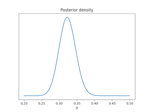
Now we can say in clear conscience that there is a 94% posterior probability that θ is in the interval (0.272, 0.363).

There are a couple predictable objections at this point. First, we didn’t get exactly 95%. No, we didn’t. But we got very close.

Second, the posterior probability depends on the prior probability. However, it doesn’t depend much on the prior. Suppose you said “I’m pretty sure most people are right handed, maybe 9 out of 10, so I’m going to start with a beta(1, 9) prior.” If so, you would compute the probability of θ being in the interval (0.272, 0.373) to be 0.948. Your a priori knowledge led you to have a little more confidence a posteriori.

Commentary

The way nearly everyone interprets a frequentist confidence interval is not justified by frequentist theory. And yet it can be justified by saying if you were to treat it as a Bayesian credible interval, you’d get nearly the same result.

You can often justify an informal understanding of frequentist statistics on Bayesian grounds. Note, however, that a Bayesian interpretation would not rescue the 95% confidence interval that returns either the empty set or the real line.

Often frequentist and Bayesian analyses reach approximately the same conclusions. A Bayesian can view frequentist techniques as convenient ways to produce approximately correct Bayesian results. And a frequentist can justify using a Bayesian procedure because the procedure has good frequentist properties.

There are times when frequentist and Bayesian results are incompatible, and in that case the Bayesian results typically make more sense in my opinion. But very often other considerations, such as model uncertainty, are much more substantial than the difference between a frequentist and Bayesian analysis.

Related posts