Solving hard problems

We help companies solve hard problems in mathematics, statistics, and computing. Let’s explore how we might work together.

CCPA and expert determination

Posted on 18 January 2020 by John

California’s new CCPA (California Consumer Privacy Act) may become more like HIPAA. In particular, a proposed amendment would apply HIPAA’s standards of expert determination to CCPA.

According to this article,

The California State Senate’s Health Committee recently approved California AB 713, which would amend the California Consumer Privacy Act (CCPA) to except from CCPA requirements additional categories of health information, including data de-identified in accordance with HIPAA and certain medical research data.

Some businesses have been looking to HIPAA by analogy for how to comply with CCPA. HIPAA has been on the books much longer, and what it means to comply with HIPAA is more clearly stated, in regulation itself and in guidance documents. AB 713 would make this appeal to HIPAA more than an analogy.

In particular, CCPA would now have a notion of expert determination. AB 713 explicitly refers to

The deidentification methodology described in Section 164.514(b)(1) of Title 45 of the Code of Federal Regulations, commonly known as the HIPAA expert determination method.

Emphasis added. Taken from 1798.130 (a)(5)(D)(i).

Update: California’s governor signed AB 713 into law on September 25, 2020.

Parsing AB 713

The amendment is hard to read because it doesn’t contain many complete sentences. The portion quoted above doesn’t have a verb. We have to go to up to (a) in the hierarchy before we can find a clear subject and verb:

… a business shall …

It’s not clear to me what the amendment is saying. Rather than trying to parse this myself, I’ll quote what the article linked above says.

AB 713 would except from CCPA requirements de-identified health information when … The information is de-identified in accordance with a HIPAA de-identification method [and two other conditions].

Expert determination

I am not a lawyer; I advise lawyers on statistical matters. I offer statistical advice, not legal advice.

If your lawyer determines that you need HIPAA-style expert determination to comply with CCPA, I can help. I have provided expert determination for many companies and would welcome the opportunity to provide this service for your company as well.

If you’d like discuss expert determination, either for HIPAA or for CCPA, let’s talk.

Variation on cosine fixed point

Posted on 18 January 2020 by John

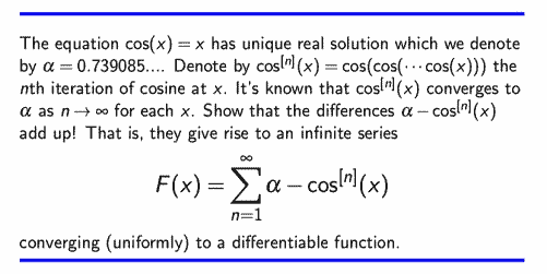
If you enter any number into a calculator and repeatedly press the cosine key, you’ll eventually get 0.73908513, assuming your calculator is in radian mode [1]. And once you get this value, taking the cosine more times won’t change the number. This is the first example of a fixed point of an iteration that many people see.

Sam Walter posted a variation on the cosine fixed point problem on Twitter recently. If you add up the distance from each iteration value to the fixed point, the sum converges. Furthermore, if you consider this sum as a function of the starting point x, it defines a differentiable function of x.

I was curious what this function looks like, so I wrote the following Python code. First we find the fixed point.

    from math import cos

    epsilon = 1e-16
    x, cx = 1, cos(1)
    while abs(x - cx) > epsilon:
        x, cx = cx, cos(cx)

    alpha = x # fixed point

Now let’s evaluate the function described above.

    def f(x):
        s = 0
        cx = cos(x)
        delta = alpha - cx
        while abs(delta) > epsilon:
            s += delta
            x, cx = cx, cos(cx)
            delta = alpha - cx
        return s

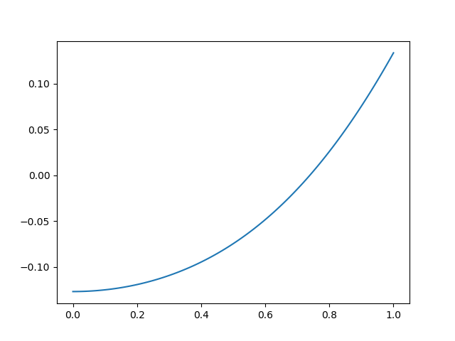
Here’s what the plot of our function looks like.

As we’d expect, it crosses the x-axis at the fixed point.

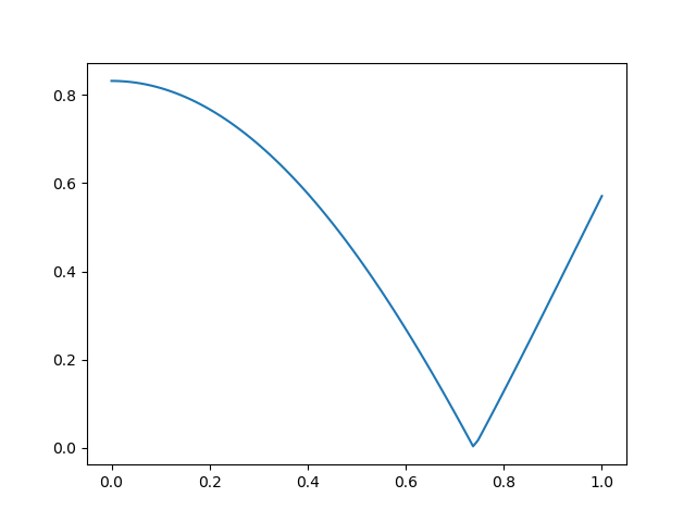
If we sum the absolute distance to the fixed point at each iteration, we get the following function with a minimum at the fixed point.

Python’s new walrus operator

Incidentally, we can make the code slightly more compact if we take advantage of a new feature in Python 3.8, affectionately known as the “walrus operator.” The := operator lets you do assignments inside a loop test, among other places, much like is commonly done in C.

    def f(x):
        s, cx = 0, cos(x)
        while abs(delta := alpha - cx) > 1e-16:
            s += delta
            x, cx = cx, cos(cx)
        return s

Now we don’t need to compute delta before the loop, and we can update delta and check its absolute value in the same place.

I’m not sure how I feel about the walrus operator. It could make code easier to read or harder to read, depending on context.

One advantage of Python’s walrus over its C analog is that it prevents bugs due to typing = when you mean to type ==. If you really want to do an assignment inside a Boolean test, you’ll need an extra character, the colon in front of the equal sign; using an ordinary equal sign alone is a syntax error.

Stable and unstable recurrence relations

Posted on 17 January 2020 by John

Mother helping her toddler to walk

The previous post looked at computing recurrence relations. That post ends with a warning that recursive evaluations may nor may not be numerically stable. This post will give examples that illustrate stability and instability.

There are two kinds of Bessel functions, denoted J and Y. These are called Bessel functions of the first and second kinds respectively. These functions carry a subscript n denoting their order. Both kinds of Bessel functions satisfy the same recurrence relation:

f_n+1 − (2n/x) f_n + f_n−1 = 0

where f is J or Y.

If you apply the recurrence relation in the increasing direction, it is unstable for J but stable for Y.

If you apply the recurrence relation in the opposite direction, it is stable for J and unstable for Y.

We will illustrate the above claims using the following Python code. Since both kinds of Bessel function satisfy the same recurrence, we pass the Bessel function in as a function argument. SciPy implements Bessel functions of the first kind as jv and Bessel functions of the second kind as yv. [1]

    from scipy import exp, pi, zeros
    from scipy.special import jv, yv

    def report(k, computed, exact):
        print(k, computed, exact, abs(computed - exact)/exact)

    def bessel_up(x, n, f):
        a, b = f(0, x), f(1, x)
        for k in range(2, n+1):
            a, b = b, 2*(k-1)*b/x - a
            report(k, b, f(k,x))     

    def bessel_down(x, n, f):
        a, b = f(n,x), f(n-1,x)
        for k in range(n-2, -1, -1):
            a, b = b, 2*(k+1)*b/x - a
            report(k, b, f(k,x))

We try this out as follows:

    bessel_up(1, 20, jv)
    bessel_down(1, 20, jv)
    bessel_up(1, 20, yv)
    bessel_down(1, 20, yv)

When we compute J_n(1) using bessel_up, the relative error starts out small and grows to about 1% when n = 9. The relative error increases rapidly from there. When n = 10, the relative error is 356%.

For n = 20, the recurrence gives a value of 316894.36 while the true value is 3.87e−25, i.e. the computed value is 30 orders of magnitude larger than the correct value!

When we use bessel_down, the results are correct to full precision.

Next we compute Y_n(1) using bessel_up the results are correct to full precision.

When we compute Y_n(1) using bessel_down, the results are about as bad as computing J_n(1) using bessel_up. We compute Y₀(1) as 0 5.7e+27 while the correct value is roughly 0.088.

There are functions, such as Legendre polynomials, whose recurrence relations are stable in either direction, at least for some range of inputs. But it would be naive to assume that a recurrence is stable without some exploration.

Miller’s algorithm

There is a trick for using the downward recurrence for Bessel functions known as Miller’s algorithm. It sounds crazy at first: Assume J_N(x) = 1 and J_N+1(x) = 0 for some large N, and run the recurrence downward.

Since we don’t know J_N(x) our results be off by some constant proportion. But there’s a way to find out what that proportionality constant is using the relation described here.

$1 = J_0(x) + 2J_2(x) + 2J_4(x) + 2J_6(x) + \cdots$

We add up out computed values for the terms on the right side, then divide by the sum to normalize our estimates. Miller’s recurrence algorithm applies more generally to other recurrences where the downward recurrence is stable and there exists a normalization identity analogous to the one for Bessel functions.

The following code lets us experiment with Miller’s algorithm.

    def miller(x, N):
        j = zeros(N) # array to store values
        
        a, b = 0, 1
        for k in range(N-1, -1, -1):
            a, b = b, 2*(k+1)*b/x - a
            j[k] = b
            
        norm = j[0] + sum(2*j[k] for k in range(2,N,2))
        j /= norm
        
        for k in range(N-1, -1, -1):
            expected, computed = j[k], jv(k,x)
            report(k, j[k], jv(k,x))

When we call miller(pi, 20) we see that Miller’s method computes J_n(π) accurately. The error starts out moderately small and decreases until the results are accurate to floating point precision.

    |----+------------|
    |  k | rel. error |
    |----+------------|
    | 19 |   3.91e-07 |
    | 17 |   2.35e-09 |
    | 16 |   2.17e-11 |
    | 15 |   2.23e-13 |
    | 14 |   3.51e-15 |
    |----+------------|

For smaller k the relative error is also around 10⁻¹⁵, i.e. essentially full precision.

[1] Why do the SciPy names end in “v”? The order of a Bessel function does not have to be an integer. It could be any real number, and the customary mathematical notation is to use a Greek letter ν (nu) as a subscript rather than n as a reminder that the subscript might not represent an integer. Since a Greek ν looks similar to an English v, SciPy uses v as a sort of approximation of ν.

Recurrence relations and Python

Posted on 17 January 2020 by John

A video by Raymond Hettinger points out that simultaneous assignment makes it much easier to understand code that evaluates a recurrence relation. His examples were in Python, but the same principle applies to any language supporting simultaneous evaluation.

The simplest example of simultaneous evaluation is swapping two variables:

   a, b = b, a

Compare this to

    temp = a
    a = b
    b = temp

The latter is more code, but more importantly it exposes intermediate steps that could be confusing if the code were more complicated. This is the case when evaluating recurrence relations.

The most famous recurrence relation is the Fibonacci sequence, but I’ll use a difference example because Fibonacci is overdone. Also, I think it helps to see a slightly more complicated example.

As I wrote earlier here, the first two Hermite polynomials are given by H₀(x) = 1 and H₁(x) = x. The rest are given via the recurrence relation

H_n+1(x) = x H_n – n H_n−1(x).

If we have a particular value of x, say x = 3, and we want to find H₁₀(x) we could do so as follows.

    x = 3
    a, b = 1, x
    for n in range(2, 11):
        a, b = b, x*b - n*a

After this code runs, b will contain H₁₀(3). [1]

At each iteration, the calculations on the right side of the equal sign are carried out, then the assignments to the elements on the left side are made. You don’t have to write explicit and confusing code with variables like a_old and a_new.

Three-term recurrence relations come up constantly in application. For example, all orthogonal polynomials satisfy some three-term recurrence analogous to the one given above for Hermite polynomials.

Power series solutions for differential equations lead to recurrence relations for the coefficients. Second order ODEs give rise to three-term recurrence relations. In general nth order ODEs give rise to n+1 term relations. By far the most common value of n in application is 2, but higher values come up occasionally.

A third-order ODE that leads to a four-term recurrence could be implemented in Python with code of the form

   a, b, c = b, c, f(a,b,c)

See this post for an example of a recently discovered three-term recurrence relation.

One final comment on recurrence relations: recurrences that hold in theory may not be useful in practice. Repeated evaluation of a recurrence might have problems with numerical stability. That’s the topic for the next post.

***

[1] If you’re not used to Python’s range generator, you might be surprised that the second argument is 11 rather than 10. This is because range(a,b) uses half-open intervals, i.e. it generates values n with a ≤ n < b. This has its advantages. For example, it composes well under unions: the union of range(a,b) and range(b,c) is range(a,c). This wouldn’t be the case if range returns its upper limit.

Reminder of complexity

Posted on 16 January 2020 by John

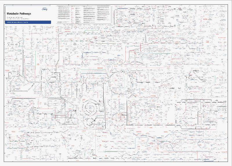
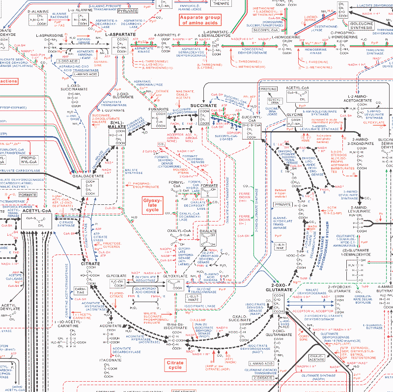
The other day I ran across the biochemical pathways poster from Roche.

biochemical pathways thumbnail

This is the first of two posters. Both posters are about 26 square feet in area. Below is a close up of about one square foot in the middle of the first poster.

middle of b8ochemical pathways poster

I’d seen this before, I think while I was working at MD Anderson Cancer Center, and it’s quite an impressive piece of work. A lot of work went into the production of the posters themselves, but the amount of hard-won knowledge the posters represent is mind-boggling. One little arrow on one poster might represent a career’s work.

A paper distributed with the charts explains that the pathways included represent a small selection of what is known.

Some indication of the degree of selection can be taken from the fact that in the present “Pathways” about 1,000 enzymes are shown. … Estimations of the number of proteins (with and without enzymatic activity) in a single mammalian cell are in the order of magnitude of 30,000.

I told a friend that I was thinking about getting a copy of the poster as a reminder of complexity, an analog of a memento mori meant to serve as a reminder of one’s mortality. The Latin phrase memento mori means “remember that you must die.” The biochemical pathways makes me thing “remember that you are complex” or “remember the world is complex.”

I asked a Latin scholar what an appropriate aphorism would be, and she suggested the phrase memento complexitatis, which translates as “be mindful of complexity.” Another suggestion was omnia contexta sunt, meaning “all things have been braided.” As Rich Hickey explains in his popular video, complex literally means braided together.

Everything impacts everything. Independence is always a simplifying assumption. The assumption may be justified, but it is an assumption.

The poster is also a reminder that we need not throw up our hands in the face of complexity. Often the implication of mathematical discussions of complexity is that predicting the future is hopeless; there’s no point trying to understand the behavior of a complex system except in some abstract qualitative way. The Roche posters are inspiring reminders that with hard work, we can learn something about complex systems. In fact, over time we can learn quite a lot.

Logistic trajectories

Posted on 16 January 2020 by John

This post is a follow-on to the post on how to make the logistic bifurcation diagram below.

logistic bifurcation diagram

That post plotting the attractors for iterations of

f(x) = r x(1 – x).

This post will plot a few trajectories over time for differing starting points and varying values of r.

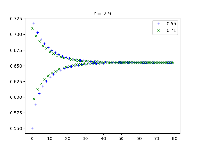
For values of r less than 3, the iterations converge to the same point regardless of where they start. The fixed point only depends on r. In the plot below, r = 2.9. We start from two different initial points, x = 0.55 and x = 0.71. Both trajectories oscillate toward a common limiting value. (As explained in the earlier post, the limiting value is (r − 1)/r = 0.6786.)

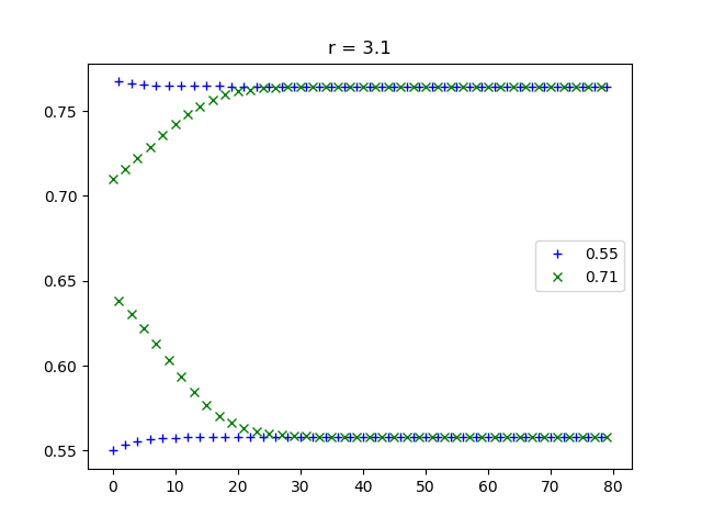
For values of r a little greater than 3, the iterations oscillate between two values. Here we chose r = 3.1, and again we start from x = 0.55 and x = 0.71.

two-point attractor

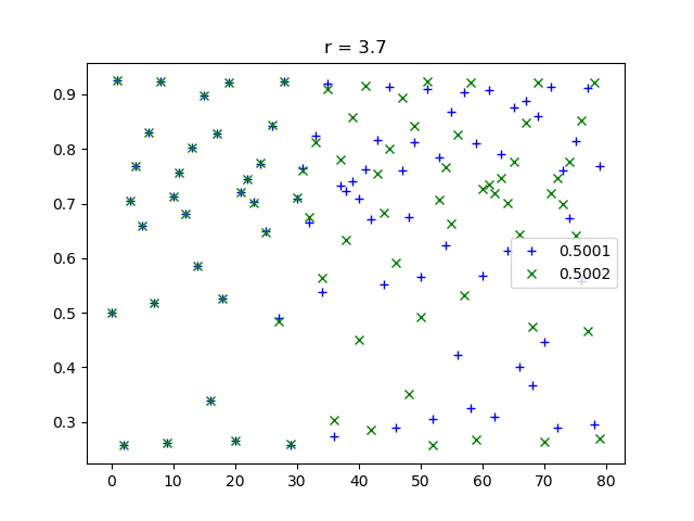
For some larger value of r the iterations rotate between four values, then eight, etc. But for even larger values of r the trajectories are chaotic. Nearby starting points lead to divergent iterations. In the plot below, r = 3.7, which is in the chaotic region. We start with points close to each other, x = 0.5001 and x = 0.5002.

chaotic trajectories

Notice how the blue crosses and green x’s are on top of each other for the first 30 iterations or so, then they diverge.

These plots were created using the following Python code.

import numpy as np
import matplotlib.pyplot as plt

def f(x, r):
    return r*x*(1-x)

def time_plot(x0, y0, r, name):
    N = 80
    x = np.zeros(N)
    y = np.zeros(N)
    x[0] = x0
    y[0] = y0
    for i in range(1,N):
        x[i] = f(x[i-1], r)
        y[i] = f(y[i-1], r)

    t = np.arange(N)
    plt.plot(t, x, "b+")
    plt.plot(t, y, "gx")
    plt.legend([str(x0), str(y0)])
    plt.title(f"r = {r}")
    plt.savefig(name)
    plt.close()

Analogies between Weierstrass functions and trig functions

Posted on 15 January 2020 by John

If you look at the Wikipedia article on Weierstrass functions, you’ll find a line that says “the relation between the sigma, zeta, and ℘ functions is analogous to that between the sine, cotangent, and squared cosecant functions.” This post unpacks that sentence.

Weierstrass p function

First of all, what is ℘? It’s the Weierstrass elliptic function, which is the mother of all elliptic functions in some sense. All other elliptic functions can be constructed from this function and its derivatives. As for the symbol itself, ℘ is the traditional symbol for the Weierstrass function. It’s U+2118 in Unicode, &weierp; in HTML, and \wp in LaTeX.

The line above suggests that ℘(x) is analogous to csc²(x). Indeed, the plots of the two functions are nearly identical.

Here’s Weierstrass’ function:

Weierstrass p plot

And here’s csc²:

plot of csc^2

The two plots basically agree to within the thickness of a line.

The Weierstrass function ℘ has two parameters that I haven’t mentioned. Elliptic functions are periodic in two directions in the complex plane, and so their values everywhere are determined by their values over a parallelogram. The two parameters specify the fundamental parallelogram, or at least that’s one way of parametrizing the function. The WeierstrassP function in Mathematica takes two other parameters, called the invariants, and these invariants were chosen in the plot above to match the period of the cosecant function.

    Plot[Sin[x]^-2, {x, -10, 10}]
    Plot[WeierstrassP[
            x, 
            WeierstrassInvariants[{Pi/2, Pi I/2}]
         ], 
        {x, -10, 10}
    ]

The fundamental parallelogram is defined in terms of half periods, usually denoted with ω’s, and the invariants are denoted with g‘s. The function WeierstrassInvariants converts from half periods to invariants, from ω’s to g‘s.

Note that ℘ and cosecant squared are similar along the real axis, but they’re very different in the full complex plane. Trig functions are periodic along the real axis but grow exponentially along the complex axis. Elliptic functions are periodic along both axes.

Weierstrass zeta function

The Weierstrass zeta function is not an elliptic function. It is not periodic but rather quasiperiodic. The derivative of the Weierstrass zeta function is negative of the Weierstrass elliptic function, i.e.

ζ ‘(x) = -℘(x)

which is analogous to the fact that the derivative of cot(x) is -csc²(x). So in that sense ζ is to ℘ as cotangent is to cosecant squared.

The plots of ζ(x) and cot(x) are similar as shown below.

Plot of Weierstrass zeta and cotangent

The Mathematica code to make the plot above was

    Plot[
        {WeierstrassZeta[x, WeierstrassInvariants[{Pi/2, Pi I/2}]], 
         Cot[x]}, 
        {x, -10, 10}, 
        PlotLabels -> {"zeta", "cot"}
    ]

Weierstrass sigma function

The Weierstrass sigma function is also not an elliptic function. It is analogous to the sine function as follows. The logarithmic derivative of the Weierstrass sigma function is the Weierstrass zeta function, just as the logarithmic derivative of sine is cotangent. That is,

(log(σ(x))’ = ζ(x).

The logarithmic derivative of a function is the derivative of its log, and so the logarithmic derivative of a function f is f ‘ / f.

However, the plot of the sigma function, WeierstrassSigma in Mathematica, hardly looks line sine.

Plot of Weierstrass sigma and sine

So in summary, logarithmic derivative takes Weierstrass sigma to Weierstrass zeta just as it takes sine to cotangent. Negative derivative takes Weierstrass zeta to Weierstrass ℘ just as it takes cotangent to negative cosecant squared.

More efficient way to sum a list comprehension

Posted on 15 January 2020 by John

List comprehensions in Python let you create a list declaratively, much like the way you would describe the set in English. For example,

    [x**2 for x in range(10)]

creates a list of the squares of the numbers 0 through 9.

If you wanted the sum of these numbers, you could of course say

    sum( [x**2 for x in range(10)] )

but in this case the brackets are unnecessary. The code is easier to read and more efficient if you omit the brackets.

    sum( x**2 for x in range(10) )

With the brackets, Python constructs the list first then sums the elements. Without the brackets, you have a generator expression. Python will sum the values as they’re generated, not saving all the values in memory. This makes no difference for a short list as above, but with a large list comprehension the generator expression could be more efficient.

On this day

Posted on 14 January 2020 by John

I looked back to see what posts I had written on this date in years past. January 14 doesn’t have any particular significance for me, so these post are a representative cross section of the blog.

Some years I didn’t write anything on January 14, and some years I wrote posts that are not worth revisiting. Here are some posts that have held up well.

On this day in 2008 I wrote about four tips for learning regular expressions. I keep writing about regular expressions occasionally. Readers find them interesting, in part because they’re useful, but perhaps also because they’re fairly simple but not trivial. There are little complications and subtleties in how they’re used.

On this day in 2009 I wrote about how to display figures side by side in LaTeX. I often get one of two responses when I write about LaTeX. The first is “Thanks. That’s what I needed. Now I can get on with my work.” The other is “That’s not the latest way to do things!” I have updated my LaTeX habits over the years, but I’m not ashamed to use older syntax if it produces the same array of pixels in the end.

On this day in 2011 I commented on conversations that can be summarized as “Your job is trivial. (But I couldn’t do it.)” The explicit message is “I could do this myself” while the implicit message is “There’s no way I could do this myself, and so I desperately need you to do it for me.”

(You’ll find several older posts on the frustrations of working inside a large bureaucratic institution. These posts stopped suddenly around the beginning of 2013 for some reason.)

On this day in 2013 I riffed on a line from Dune about adaptive decision making. The next day I announced here that I was leaving my job to start my consultancy.

On this day in 2015 I elaborated on a someone’s remark that “the result of striving for ultimate simplicity is intolerable complexity.” I’ve seen that over and over, especially in software projects. A moderate desire for simplicity makes things simpler. But when people obsess on a particular notion of simplicity, they can make things horribly complex. These are often very smart people; they make things difficult in a way that less intelligent people couldn’t pull off.

On this day last year I wrote about algorithms for multiplying very large numbers. This is a practical question in cryptography, for example, but there have been recent theoretical developments which are interesting but as yet impractical.

I wonder what I might be writing about this time next year, assuming I’m still around and still blogging. Probably something about applied math; I write about math more often than the sampling above would imply. Maybe I’ll write something about computing or privacy, topics I’ve written about more often recently.

Thanks for reading.

Logistic bifurcation diagram in detail

Posted on 11 January 2020 by John

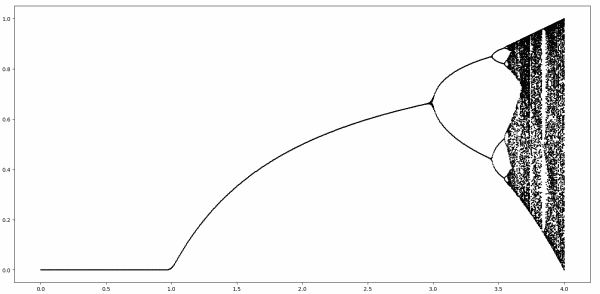
The image below is famous. I’ve seen it many times, but rarely with a detailed explanation. If you’ve ever seen this image but weren’t sure exactly what it means, this post is for you.

logistic bifurcation diagram

This complex image comes from iterating a simple function

f(x) = r x(1 − x)

known as the logistic map. The iterates of the function can behave differently for different values of the parameter r.

We’ll start by fixing a value of r, with 0 ≤ r < 1. For any starting point 0 ≤ x ≤ 1, f(x) is going to be smaller than x by at least a factor of r, i.e.

0 ≤ f(x) ≤ rx.

Every time we apply f the result decreases by a factor of r.

0 ≤ f( f(x) ) ≤ r²x.

As we do apply f more and more times, the result converges to 0.

For r ≥ 1 it’s not as clear what will happen as we iterate f, so let’s look at a little bit of code to help see what’s going on.

    def f(x, r):
        return r*x*(1-x)

    def iter(x, r, n):
        for _ in range(n):
            x = f(x, r)
        return x

We can see that for 1 ≤ r ≤ 3, and 0 ≤ x ≤ 1, the iterations of f converge to a fixed point, and the value of that fixed point increases with r.

    >>> iter(0.1, 1.1, 100)
    0.09090930810626502

    # more iterations have little effect
    >>> iter(0.1, 1.1, 200)
    0.09090909091486

    # different starting point has little effect
    >>> iter(0.2, 1.1, 200)
    0.0909090909410433

    # increasing r increases the fixed point
    >>> iter(0.2, 1.2, 200)
    0.16666666666666674

Incidentally, for 1 ≤ r ≤ 3, the fixed point equals (r − 1)/r. [1]

When r is a little bigger than 3, things get more interesting. Instead of a single fixed point, the iterates alternate between a pair of points, an attractor consisting of two points.

    >>> iter(0.2, 3.1, 200) 
    0.7645665199585945  
                             
    >>> iter(0.2, 3.1, 201) 
    0.5580141252026958  
                             
    >>> iter(0.2, 3.1, 202) 
    0.7645665199585945

How can we write code to detect an attractor? We can look at the set of points when we get, say when we iterate 1000, then 1001, etc. up to 1009 times. If this set has less than 10 elements, the iterates must have returned to one of the values. We’ll round the elements in our set to four digits so we actually get repeated values, not just values that differ by an extremely small amount.

    def attractors(x, r):
        return {round(iter(x, r, n), 4) for n in range(1000,1010)}

This is crude but it’ll do for now. We’ll make it more efficient, and we’ll handle the possibility of more than 10 points in an attractor.

Somewhere around r = 3.5 we get not just two points but four points.

    >>> attractors(0.1, 3.5)
    {0.3828, 0.5009, 0.8269, 0.875}

As r gets larger the number of points keeps doubling [2] until chaos sets in.

The function attractors is simple but not very efficient. After doing 1000 iterations, it starts over from scratch to do 1001 iterations etc. And it assumes there are no more than 10 fixed points. The following revision speeds things up significantly.

    def attractors2(x, r):
        x = iter(x, r, 100)
        x0 = round(x, 4)
        ts = {x0}
        for c in range(1000):
            x = f(x, r)
            xr = round(x, 4)
            if xr in ts:
                return ts
            else:
                ts.add(xr)

Notice we put a cap of 1000 on the number of points in the attractor for a given r. For some values of r and x, there is no finite set of attracting points.

Finally, here’s the code that produced the image above.

    import numpy as np
    import matplotlib.pyplot as plt
    rs = np.linspace(0, 4, 1000)
    for r in rs:
        ts = attractors2(0.1, r)
        for t in ts:
            plt.plot(r, t, "ko", markersize=1)
    plt.show()

Update: See this post for graphs showing the trajectory of points over time for varying values of r.