Scaled Beta2 distribution

I recently ran across a new probability distribution called the “Scaled Beta2” or “SBeta2” for short in [1].

For positive argument x and for positive parameters p, q, and b, its density is

\frac{\Gamma(p+q)}{b\,\Gamma(p) \, \Gamma(q)}\, \frac{\left(\frac{x}{b}\right)^{p-1}}{\left(\left(\frac{x}{b}\right) + 1 \right)^{p+q}}

This is a heavy-tailed distribution. For large x, the probability density is O(xq−1), the same as a Student-t distribution with q degrees of freedom.

The authors in [1] point out several ways this distribution can be useful in application. It can approximate a number of commonly-used prior distributions while offering advantages in terms of robustness and analytical tractability.

Related posts

[1] The Scaled Beta2 Distribution as a Robust Prior for Scales. María-Eglée Pérez, Luis Raúl Pericchi, Isabel Cristina Ramírez. Available here.

Applications of (1−z)/(1+z)

I keep running into the function

f(z) = (1 − z)/(1 + z).

The most recent examples include applications to radio antennas and mental calculation. More on these applications below.

Involutions

A convenient property of our function f is that it is its own inverse, i.e. f( f(x) ) = x. The technical term for this is that f is an involution.

The first examples of involutions you might see are the maps that take x to −x or 1/x, but or function shows that more complex functions can be involutions as well. It may be the simplest involution that isn’t obviously an involution.

By the way, f is still an involution if we extend it by defining f(−1) = ∞ and f(∞) = −1. More on that in the next section.

Möbius transformations

The function above is an example of a Möbius transformation, a function of the form

(az + b)/(cz + d).

These functions seem very simple, and on the surface they are, but they have a lot of interesting and useful properties.

If you define the image of the singularity at z = −d/c to be ∞ and define the image of ∞ to be a/c, then Möbius transformations are one-to-one mappings of the extended complex plane, the complex numbers plus a point at infinity, onto itself. In fancy language, the Möbius transformations are the holomorphic automorphisms of the Riemann sphere.

More on why the extended complex plane is called a sphere here.

One nice property of Möbius transformations is that they map circles and lines to circles and lines. That is, the image of a circle is either a circle or a line, and the image of a line is either a circle or a line. You can simplify this by saying Möbius transformations map circles to circles, with the understanding that a line is a circle with infinite radius.

Electrical engineering application

Back to our particular Möbius transformation, the function at the top of the post.

I’ve been reading about antennas, and in doing so I ran across the Smith chart. It’s essentially a plot of our function f. It comes up in the context of antennas, and electrical engineering more generally, because our function f maps reflection coefficients to normalized impedance. (I don’t actually understand that sentence yet but I’d like to.)

The Smith chart was introduced as a way of computing normalized impedance graphically. That’s not necessary anymore, but the chart is still used for visualization.

Smith chart

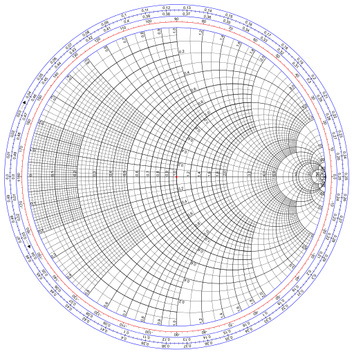
Image Wdwd, CC BY-SA 3.0, via Wikimedia Commons.

Mental calculation

It’s easy to see that

f(a/b) = (ba)/(b + a)

and since f is an involution,

a/b = f( (b − a)/(b + a) ).

Also, a Taylor series argument shows that for small x,

f(x)nf(nx).

A terse article [1] bootstraps these two properties into a method for calculating roots. My explanation here is much longer than that of the article.

Suppose you want to mentally compute the 4th root of a/b. Multiply a/b by some number you can easily take the 4th root of until you get a number near 1. Then f of this number is small, and so the approximation above holds.

Bradbury gives the example of finding the 4th root of 15. We know the 4th root of 1/16 is 1/2, so we first try to find the 4th root of 15/16.

(15/16)1/4 = f(1/31)1/4f(1/124) = 123/125

and so

151/4 ≈ 2 × 123/125

where the factor of 2 comes from the 4th root of 16. The approximation is correct to four decimal places.

Bradbury also gives the example of computing the cube root of 15. The first step is to multiply by the cube of some fraction in order to get a number near 1. He chooses (2/5)3 = 8/125, and so we start with

15 × 8/125 = 24/25.

Then our calculation is

(24/25)1/3 = f(1/49)1/3f(1/147) = 73/74

and so

151/3 ≈ (5/2) × 73/74 = 365/148

which is correct to 5 decimal places.

Update: See applications of this transform to mentally compute logarithms.

[1] Extracting roots by mental methods. Robert John Bradbury, The Mathematical Gazette, Vol. 82, No. 493 (Mar., 1998), p. 76.

Saxophone ranges

Saxophone quartet

I stumbled on a recording of a contrabass saxophone last night and wondered just how low it was [1], so I decided to write this post giving the ranges of each of the saxophones.

The four most common saxophones are baritone, tenor, alto, and soprano. These correspond to the instruments in the image above. There are saxophones below the baritone and above the soprano, but they’re rare.

Saxophones have roughly the same range as the human vocal parts with the corresponding names, as shown in the following table.

\begin{center} \begin{tabular}{lllrr} \hline Part & Sax SPN & Human SPN & Sax Hz & Human Hz\\ \hline Soprano & \(A \flat_3\) -- \(E \flat_6\) & \(C_4\) -- \(C_6\) & 208--1245 & 262--1047\\ Alto & \(D \flat_3\) -- \(A \flat_5\) & \(F_3\) -- \(F_5\) & 139--831 & 175--698\\ Tenor & \(A \flat_2\) -- \(E \flat_5\) & \(C_3\) -- \(C_5\) & 104--622 & 131--523\\ Baritone & \(D \flat_2\) -- \(A \flat_4\) & \(G_2\) -- \(G_4\) & 69--415 & 98--392\\ Bass & \(A \flat_1\) -- \(E \flat_4\) & \(E_2\) -- \(E_4\) & 52--311 & 82--330\\ \hline \end{tabular} \end{center}

SPN stands for scientific pitch notation, explained here. Hz stands for Hertz, vibrations per second.

The human ranges are convenient two-octave ranges. Of course different singers have different ranges. (Different saxophone players have different ranges too if you include the altissimo range.)

If you include the rare saxophones, the saxophone family has almost the same range as a piano. The lowest note on a subcontrabass saxophone is a half step lower than the lowest note on a piano, and the highest note on the sopranissimo saxophone is a few notes shy of the highest note on a piano.

\begin{center} \begin{tabular}{llr} \hline Part & Sax SPN & Sax Hz\\ \hline Sopranissimo & \(A \flat_4\) -- \(E \flat_7\) & 416--2490\\ Sopranino & \(D \flat_4\) -- \(A \flat_6\) & 277--1662\\ Soprano & \(A \flat_3\) -- \(E \flat_6\) & 208--1245\\ Alto & \(D \flat_3\) -- \(A \flat_5\) & 139--831\\ Tenor & \(A \flat_2\) -- \(E \flat_5\) & 104--622\\ Baritone & \(D \flat_2\) -- \(A \flat_4\) & 69--415\\ Bass & \(A \flat_1\) -- \(E \flat_4\) & 52--311\\ Contrabass & \(D \flat_1\) -- \(A \flat_3\) & 35--208\\ Subcontrabass & \(A \flat_0\) -- \(E \flat_3\) & 26--156\\ \hline \end{tabular} \end{center}

Update

My intent when I wrote this post was to add some visualization. One thought was to display the data above on a piano keyboard. That would be a nice illustration, but it would be a lot of work to create. Then it occurred to me that what putting things on a piano is really just a way of displaying the data on a log scale. So I plotted the frequency data on a log scale, which was much easier.

Saxophone and human voice ranges

More saxophone posts

[1] I could figure it out in terms of musical notation—you can see what a regular pattern the various saxes have in the table above—but I think more in terms of frequencies these days, so I wanted to work everything out in terms of Hz. Also, I’d always assumed that tenor saxes and tenor voices have about the same range etc., but I hadn’t actually verified this before.

Fraction comparison trick

If you want to determine whether

a/b > c/d,

it is often enough to test whether

a + d > b + c.

Said another way a/b is usually greater than c/d when a + d is greater than b + c.

This sounds imprecise if not crazy. But it is easy to make precise and [1] shows that it is true.

Examples

Consider 4/11 vs 3/7. In this case 4 + 7 = 11 < 11 + 3 = 14, which suggests 4/11 < 3/7, which is correct.

But the rule of thumb can lead you astray. For example, suppose you want to compare 3/7 and 2/5. We have 3 + 5 = 8 < 7 + 2 = 9, but 3/7 > 2/5.

The claim isn’t that the rule always works; clearly it doesn’t. The claim is that it usually works, in a sense that will be made precise in the next section.

Rigorous statement

Let N be a large integer, and pick integers a, b, c, and d at random uniformly between 1 and N. Let

x = a/bc/d

and

y = (a+d) − (b+c).

Then the probability x and y are both positive, or both negative, or both zero, approaches 11/12 as N goes to infinity.

Simulation

I won’t repeat the proof of the theorem above; see [1] for that. But I’ll give a simulation that illustrates the theorem.

    import numpy as np
    
    np.random.seed(20210225)
    
    N = 1_000_000
    numreps = 10_000
    
    count = 0
    for _ in range(numreps):
        (a, b, c, d) = np.random.randint(1, N+1, 4, dtype=np.int64)
        x = a*d - b*c
        y = (a+d) - (b+c)
        if np.sign(x) == np.sign(y):
            count += 1
    print(count/numreps)

This prints 0.9176, and 11/12 = 0.91666….

The random number generator randint defaults to 32-bit integers, but this could lead to overflow since 106 × 106 > 232. So I used 64-bit integers.

Instead of computing a/bc/d, I multiply by bd and compute adbc instead because this avoids any possible floating point issues.

In case you’re not familiar with the sign function, it returns 1 for positive numbers, 0 for 0, and −1 for negative numbers.

The code suggests a different statement of the theorem: if you generate two pairs of integers, their sums and their products are probably ordered the same way.

Psychology

This post has assumed that the numbers a, b, c, and d are all chosen uniformly at random. But the components of the fractions for which you have any doubt whether a/b is greater or less than c/d are not uniformly distributed. For example, consider 17/81 versus 64/38. Clearly the former is less than 1 and the latter is greater than 1.

It would be interesting to try to assess how often the rule of thumb presented here is correct in practice. You might try to come up with a model for the kinds of fractions people can’t compare instantly, such as proper fractions that have similar size.

Related posts

[1] Kenzi Odani. A Rough-and-Ready Rule for Fractions. The Mathematical Gazette, Vol. 82, No. 493 (Mar., 1998), pp. 107-109

Normal probability fixed point

Let Z be a standard normal random variable. Then there is a unique x such that

Pr(Z < x) = x.

That is, Φ has a unique fixed point where Φ is the CDF of a standard normal.

It’s easy to find the fixed point: start anywhere and iterate Φ.

Here’s a cobweb plot that shows how the iterates converge, starting with −2.

Cobweb plot for normal CDF

The black curve is a plot of Φ. The blue stairstep is a visualization of the iterates. The stairstep pattern comes from outputs turning into inputs. That is, vertical blue lines connect and input value x to its output value y, and the horizontal blue lines represent sliding a y value over to the dotted line y = x in order to turn it into the next x value.

y‘s become x‘s. The blue lines get short when we’re approaching the fixed point because now the outputs approximately equal the inputs.

Here’s a list of the first 10 iterates.

    0.02275
    0.50907
    0.69465
    0.75636
    0.77528
    0.78091
    0.78257
    0.78306
    0.78320
    0.78324

So it seems that after 10 iterations, we’ve converged to the fixed point in the first four decimal places.

The time-traveling professor

Suppose you were a contemporary professor sent back in time. You need to continue your academic career, but you can’t let anyone know that you’re from the future. You can’t take anything material with you but you retain your memories.

At first thought you might think you could become a superstar, like the musician in the movie Yesterday who takes credit for songs by The Beatles. But on second thought, maybe not.

Maybe you’re a physicist and you go back in time before relativity. If you go back far enough, people will not be familiar with the problems that relativity solves, and your paper on relativity might not be accepted for publication. And you can’t just post it on arXiv.

If you know about technology that will be developed, but you don’t know how to get there using what’s available in the past, it might not do you much good. Someone with a better knowledge of the time’s technology might have the advantage.

If you’re a mathematician and you go back in time 50 years, could you scoop Andrew Wiles on the proof of Fermat’s Last Theorem? Almost certainly not. You have the slight advantage of knowing the theorem is true, whereas your colleagues only strongly suspect that it’s true. But what about the proof?

If I were in that position, I might think “There’s something about a Seaborn group? No, that’s the Python library. Selmer group? That sounds right, but maybe I’m confusing it with the musical instrument maker. What is this Selmer group anyway, and how does it let you prove FLT?”

Could Andrew Wiles himself reproduce the proof of FTL without access to anything written after 1971? Maybe, but I’m not sure.

In your area of specialization, you might be able to remember enough details of proven results to have a big advantage over your new peers. But your specialization might be in an area that hasn’t been invented yet, and you might know next to nothing about areas of research that are currently in vogue. Maybe you’re a whiz at homological algebra, but that might not be very useful in a time when everyone is publishing papers on differential equations and special functions.

There are a few areas where a time traveler could make a big splash, areas that could easily have been developed much sooner but weren’t. For example, the idea of taking the output of a function and sticking it back in, over and over, is really simple. But nobody looked into it deeply until around 50 years ago.

Then came the Mandelbrot set, Feigenbaum’s constants, period three implies chaos, and all that. A lack of computer hardware would be frustrating, but not insurmountable. Because computers have shown you what phenomena to look for, you could go back and reproduce them by hand.

In most areas, I suspect knowledge of the future wouldn’t be an enormous advantage. It would obviously be some advantage. Knowing which way a conjecture was settled tells you whether to try to prove or disprove it. In the language of microprocessors, it gives you good branch prediction. And it would help to have patterns in your head that have turned out to be useful, even if you couldn’t directly appeal to these patterns without blowing your cover. But I suspect it might make you something like 50% more productive, not enough to turn an average researcher into a superstar.

The debauch of indices

This morning I was working on a linear algebra problem for a client that I first solved by doing calculations with indices. As I was writing things up I thought of the phrase “the debauch of indices” that mathematicians sometimes use to describe tensor calculations. The idea is that calculations with lots of indices are inelegant and that more abstract arguments are better.

The term “debauch of indices” pejorative, but I’ve usually heard it used tongue-in-cheek. Although some people can be purists, going to great lengths to avoid index manipulation, pragmatic folk move up and down levels of abstraction as necessary to get their work done.

I searched on the term “debauch of indices” to find out who first said it, and found an answer on Stack Exchange that traces it back to Élie Cartan. Cartan said that although “le Calcul différentiel absolu du Ricci et Levi-Civita” (tensor calculus) is useful, “les débauches d’indices” could hide things that are easier to see geometrically.

After solving my problem using indices, I went back and came up with a more abstract solution. Both approaches were useful. The former cut through a complicated problem formulation and made things more tangible. The latter revealed some implicit pieces of the puzzle that needed to be made explicit.

Related posts

Not-to-do list

There is an apocryphal [1] story that Warren Buffett once asked someone to list his top 25 goals in order. Buffett then told him that he should avoid items 6 through 25 at all costs. The idea is that worthy but low-priority goals distract from high-priority goals.

Paul Graham wrote something similar about fake work. Blatantly non-productive activity doesn’t dissipate your productive energy as unimportant work does.

I have a not-to-do list, though it’s not as rigorous as the “avoid at all costs” list that Buffett is said to have recommended. These are not hard constraints, but more like what optimization theory calls soft constraints, more like stiff springs than brick walls.

One of the things on my not-to-do list is work with students. They don’t have money, and they often want you to do their work for them, e.g. to write the statistical chapter of their dissertation. It’s easier to avoid ethical dilemmas and unpaid invoices by simply turning down such work. I haven’t made exceptions to this one.

My softest constraint is to avoid small projects, unless they’re interesting, likely to lead to larger projects, or wrap up quickly. I’ve made exceptions to this rule, some of which I regret. My definition of “small” has generally increased over time.

I like the variety of working on lots of small projects, but it becomes overwhelming to have too many open projects at the same time. Also, transaction costs and mental overhead are proportionally larger for small projects.

Most of my not-to-do items are not as firm as my prohibition against working with students but more firm than my prohibition against small projects. These are mostly things I have pursued far past the point of diminishing return. I would pick them back up if I had a reason, but I’ve decided not to invest any more time in them just-in-case.

Sometimes things move off my not-to-do list. For example, Perl was on my not-to-do list for a long time. There are many reasons not to use Perl, and I agree with all of them in context. But nothing beats Perl for small text-munging scripts for personal use.

I’m not advocating my personal not-to-do list, only the idea of having a not-to-do list. And I’d recommend seeing it like a storage facility rather than a landfill: some things may stay there a while then come out again.

I’m also not advocating evaluating everything in terms of profit. I do lots of things that don’t make money, but when I am making money, I want to make money. I might take on a small project pro bono, for example, that I wouldn’t take on for work. I heard someone say “Work for full rate or for free, but not for cheap” and I think that’s good advice.

***

[1] Some sources say this story may be apocryphal. But “apocryphal” means of doubtful origin, so it’s redundant to say something may be apocryphal. Apocryphal does not mean “false.” I’d say a story might be false, but I wouldn’t say it might be apocryphal.

Herd immunity countdown

A few weeks ago I wrote a post giving a back-of-the-envelope calculation regarding when the US would reach herd immunity to SARS-COV-2. As I pointed out repeatedly, this is only a rough estimate because it makes numerous simplifying assumptions and is based on numbers that have a lot of uncertainty around them. See that post for details.

That post was based on the assumption that 26 million Americans had been infected with the virus. I’ve heard other estimates of 50 million or 100 million.

Update: The CDC estimates that 83 million Americans were infected in 2020 alone. I don’t see that they’ve issued any updates to this figure, but everyone who has been infected in 2021 brings us closer to herd immunity.

The post was also based on the assumption that we’re vaccinating 1.3 million per day. A more recent estimate is 1.8 million per day. (Update: We’re at 2.7 million per day as of March 30, 2021.) So maybe my estimate was pessimistic. On the other hand, the estimate for the number of people with pre-existing immunity that I used may have been optimistic.

Because there is so much we don’t know, and because numbers are frequently being updated, I’ve written a little Python code to make all the assumptions explicit and easy to update. According to this calculation, we’re 45 days from herd immunity. (Update: We could be at herd immunity any time now, depending on how many people had pre-existing immunity.)

As I pointed out before, herd immunity is not a magical cutoff with an agreed-upon definition. I’m using a definition that was suggested a year ago. Viruses never [1] completely go away, so any cutoff is arbitrary.

Here’s the code. It’s Python, but you it would be trivial to port to any programming language. Just remove the underscores as thousands separators if your language doesn’t support them and change the comment marker if necessary.

US_population         = 330_000_000
num_vaccinated        =  50_500_000 # As of March 30, 2021
num_infected          =  83_100_000 # As of January 1, 2021
vaccine_efficacy      = 0.9
herd_immunity_portion = 0.70

# Some portion of the population had immunity to SARS-COV-2
# before the pandemic. I've seen estimates from 10% up to 60%.
portion_pre_immune = 0.30
num_pre_immune = portion_pre_immune*US_population

# Adjust for vaccines given to people who are already immune.
portion_at_risk = 1.0 - (num_pre_immune + num_infected)/US_population

num_new_vaccine_immune = num_vaccinated*vaccine_efficacy*portion_at_risk

# Number immune at present
num_immune = num_pre_immune + num_infected + num_new_vaccine_immune
herd_immunity_target = herd_immunity_portion*US_population

num_needed = herd_immunity_target - num_immune

num_vaccines_per_day = 2_700_000 # As of March 30, 2021
num_new_immune_per_day = num_vaccines_per_day*portion_at_risk*vaccine_efficacy

days_to_herd_immunity = num_needed / num_new_immune_per_day

print(days_to_herd_immunity)

[1] One human virus has been eliminated. Smallpox was eradicated two centuries after the first modern vaccine.

Martin’s doileys

An iteration due to artist mathematician [1] Barry Martin produces intricate doiley-like patterns by iterating a simple mathematical function. I ran across this via [2].

{x \choose y} \to {y - \text{sign}(x)\sqrt{bx -c|} \choose a - x} % pardon the non-semantic use of choose

The images produced are sensitive to small changes in the starting parameters x and y, as well as to the parameters a, b, and c.

Here are three examples:

make_plot(5, 5, 30.5, 2.5, 2.5,

make_plot(5, 6, 30, 3, 3,

make_plot(3, 4, 5, 6, 7,

And here’s the Python code that was used to make these plots.

    import matplotlib.pyplot as plt
    from numpy import sign, empty

    def make_plot(x, y, a, b, c, filename, N=20000):
        xs = empty(N)
        ys = empty(N)
        for n in range(N):
            x, y = y - sign(x)*abs(b*x - c)**0.5, a - x
            xs[n] = x
            ys[n] = y
        plt.scatter(xs, ys, c='k', marker='.', s = 1, alpha=0.5)
        plt.axes().set_aspect(1)
        plt.axis('off')
        plt.savefig(filename)
        plt.close()

    make_plot(5, 5, 30.5, 2.5, 2.5, "doiley1.png")
    make_plot(5, 6, 30, 3, 3, "doiley2.png")
    make_plot(3, 4, 5, 6, 7, "doiley3.png")

[1] Tom Crilly identified Martin as an artist in [2] and I repeated this error. Barry Martin informed me of the error in the comments below.

[2] Desert Island Theorems: My Magnificent Seven by Tony Crilly. The Mathematical Gazette, Mar., 2001, Vol. 85, No. 502 (Mar., 2001), pp. 2-12