Error in the normal approximation to the binomial distribution

The binomial distribution can often be well approximated by a normal distribution. But how can you know when the approximation will be good? Most textbooks are vague on this point, saying “n should be large” or “np should be large.” How large? Why?

These notes will look carefully at the error in the normal approximation to the binomial distribution. We will look at how the error varies as a function of the binomial parameters n and p and demonstrate how the continuity correction improves the approximation.

Central Limit Theorem

A binomial(n, p) random variable X can be thought of as the sum of n Bernoulli random variables X_i. Applying the Central Limit Theorem to this sum shows that F_X, the CDF (cumulative distribution function) of X, is approximately equal to F_Y, the CDF of a normal random variable Y with the name mean and variance as X. That is, Y has mean np and variance npq where q = 1 − p.

But how good is the approximation? The Berry-Esséen theorem gives an upper bound on the error. It says the error is uniformly bounded by C ρ/σ³√n where C is a constant less than 0.7655, ρ = E(|X_i − p|³) and σ is the standard deviation of X_i. It’s easy to calculate ρ = pq(p² + q²) and σ = √(pq) for the Bernoulli random variables X_i. Therefore the error in the normal approximation to a binomial(n, p) random variable is bounded by C(p² + q²) /√(npq).

Error as a function of n

For fixed p, the bound C(p² + q²) /√(npq) from the Berry-Esséen theorem says that the maximum error decreases proportional to 1/√n. Hence the recommendation that the approximation be used for large n.

Error as a function of p

The term (p² + q²) /√(pq) is smallest when p = 1/2. This suggests that for a given value of n, the normal approximation is best when p is near 1/2. However, the function (p² + q²) /√(pq) is unbounded as p approaches either 0 or 1.

Assume p < 1/2 (or else reverse the rolls of p and q). For 0 < p < 1/2, one can show that (p² + q²) /√(pq) < 1/√p. Therefore the approximation error is bounded by a constant times 1/√(np), hence the suggestion that np should be “large.”

So a conservative estimate on the error is 0.7655/√(np) when p < 1/2.

Examples

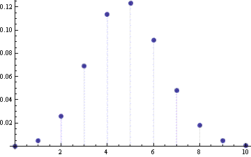
The following plot shows the error in the normal approximation to the CDF of a binomial(10, 0.5) random variable. Here we are computing F_X(n) − F_Y(n) for n = 0, 1, …, 10.

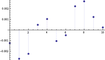
Next we compute the error again, but using the continuity correction, F_X(n) – F_Y(n+1/2).

The continuity correction lowers the maximum error from 0.123 to 0.00267, making the error 47 times smaller.

We expect the error would be larger for p = 0.1 than it was for p = 0.5 above. Indeed this is the case. For a binomial(10, 0.1) random variable, the maximum error in the normal approximation is 0.05 even when using the continuity correction.

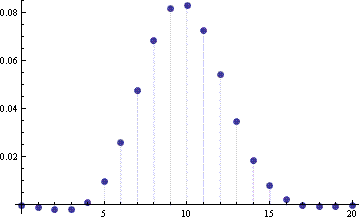
For another example we consider a binomial(100, 0.1) random variable. The following graph gives the approximation without continuity correction.

And here is the error when using the continuity correction.

In this case, n is larger and the benefit of the continuity correction is not as large. Still, the correction reduces the error by a factor of 4.8.

Approximating the PMF

Up to this point we have only looked at approximating the CDF. Now we look at approximating the probability of individual points, i.e. we look at the probability mass function (PMF).

The naive approximation would be to approximate f_X(n) with f_Y(n). However, the continuity correction requires we approximate f_X(n) by the integral

As the examples above suggest, the continuity correction greatly improves the accuracy of the approximation.

Other normal approximations

The Camp-Paulson approximation for the binomial distribution function also uses a normal distribution but requires a non-linear transformation of the argument. The result is an approximation that can be one or two orders of magnitude more accurate.

See also notes on the normal approximation to the beta, gamma, Poisson, and student-t distributions.