
It is well known that adult male heights follow a normal (Gaussian) distribution. The same is true of adult female heights. What does the distribution of adults in general look like? There are several qualitatively different answers depending on minor changes to some basic assumptions.
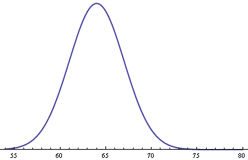
First, assume adult male heights are normally distributed with mean 70 inches and standard deviation 3 inches. Assume also that adult female heights are normally distributed with mean 64 inches and standard deviation 3 inches. These numbers are approximately correct for Americans; the averages vary by a few inches from country to country.
Under these assumptions, the probability density for a woman’s height is as follows.
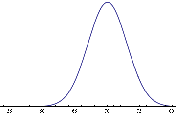
The corresponding density for men is the same, shifted to the right.
If we assume an equal number of men and women, the probability density for the height of an adult without regard to sex is given below.
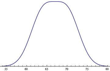
Note that this density is not Gaussian at all. Instead, it is very flat on top. You might reason that since the average of normal random variables is normal, adult heights should be normal. But we don’t have an average, we have a mixture. The density for the general adult population is a mixture of the male and female distributions. If you assigned a height to married couples as an average of the husband’s height and the wife’s height, the resulting value would be an average than a mixture and would follow a normal density.
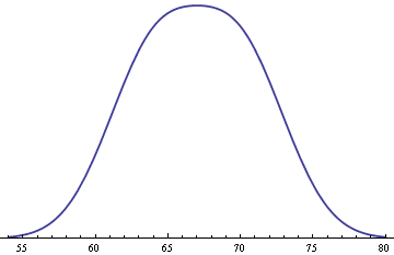
The flat top of the density above is not typical. If you have two populations with the same standard deviation and take a 50-50 mixture, the mixture will be symmetric about the average of the two population means. The second derivative of the density at the point of symmetry will be negative if the two population means are less than two standard deviations apart. For example, if the standard deviation had been 3.2 rather than 3.0, the two population means, 64 inches and 70 inches, would be less than two standard deviations apart, and the density of the mixture would be rounded at the mode of 67 inches.
The second derivative of the density will be positive in the middle if the two population means are more than two standard deviations apart. For example, if the standard deviations had been 2.8, the population means would be more than two standard deviations apart and the middle value of 67 inches would be a local minimum. (The value of 2.8 may be fairly accurate. One website I found said the standard deviation is 2.8, but I have no idea whether that site was reliable.)
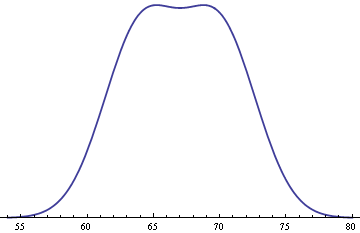
If the two population means are close to two standard deviations apart, the mixture density is still approximately flat on top, flatter than a normal density. But only when the population means are exactly two standard deviations apart is the mixture distribution completely flat on top, i.e. only then is the second derivative zero in the middle.
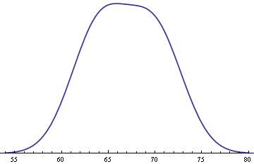
The calculations above have assumed the proportions of men and women were exactly equal. If we assume women form 51% of the population, then the density becomes slightly asymmetrical.
After this page was first posted, I found out about a couple related references.
The American Statistician had an article Is Human Height Bimodal? on this topic in 2002.
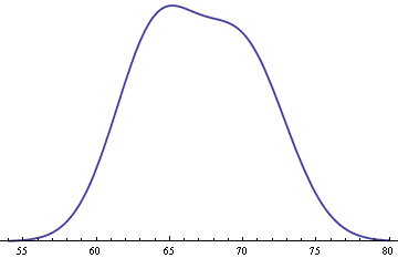
That same year Andrew Gelman and Deborah Nolan published Teaching Statistics: A Bag of Tricks which also deals with this subject. Gelman and Nolan point out that the variance of men’s heights is slightly larger than that for women. If we assume a 50-50 split of men and women, but assume male heights have a standard deviation of 3 inches while female heights have a standard deviation of 2.8 inches, this tilts the graph to the left more than assuming equal variance but unequal proportions above.
See also Why heights are normally distributed.
