Rényi’s parking constant

Parallel parking photo by IFCAR, Public Domain

Imagine parallel parking is available along the shoulder of a road, but no parking spaces are marked.

The first person to park picks a spot on the shoulder at random. Then another car also chooses a spot along the shoulder at random, with the constraint that the second car can’t overlap the first. This process continues until no more cars can park. How many people can park this way?

Assume all cars have the same length, and we choose our units so that cars have length 1. The expected number of cars that can park is a function M(x) of the length of the parking strip x. Clearly if x < 1 then M(x) = 0. Alfréd Rényi [1] found that for x ≥ 1, M(x) satisfies the equation

M(x) = 1 + \frac{2}{x-1}\int_0^{x-1} M(t)\, dt

This is an unusual equation, difficult to work with because it defined M only implicitly. It’s not even clear that the equation has a solution. But it does, and the ratio of M(x) to x approaches a constant as x increases.

m = \lim_{x\to\infty} \frac{M(x)}{x} = 0.74759\ldots

The number m is known as Rényi’s parking constant.

This say for a long parking strip, parking sequentially at random will allow about 3/4 as many cars to park as if you were to pack the cars end-to-end.

More posts on Rényi’s work

[1] Steven R. Finch. Mathematical Constants. Cambridge University Press, 2003.

Calculating when a planet will appear to move backwards

When we say that the planets in our solar system orbit the sun, not the earth, we mean that the motions of the planets is much simpler to describe from the vantage point of the sun. The sun is no more the center of the universe than the earth is. Describing the motion of the planets from the perspective of our planet is not wrong, but it is inconvenient. (For some purposes. It’s quite convenient for others.)

The word planet means “wanderer.” This because the planets appear to wander in the night sky. Unlike stars that appear to orbit the earth in a circle as the earth orbits the sun, planets appear to occasionally reverse course. When planets appear to move backward this is called retrograde motion.

Apparent motion of Venus

Here’s what the motion of Venus would look like over a period of 8 years as explored here.

Venus from Earth

Venus completes 13 orbits around the sun in the time it takes Earth to complete 8 orbits. The ratio isn’t exactly 13 to 8, but it’s very close. Five times over the course of eight years Venus will appear to reverse course for a few days. How many days? We will get to that shortly.

When we speak of the motion of the planets through the night sky, we’re not talking about their rising and setting each day due to the rotation of the earth on its axis. We’re talking about their motion from night to night. The image above is how an observer far above the Earth and not rotating with the Earth would see the position of Venus over the course of eight years.

The orbit of Venus as seen from earth is beautiful but complicated. From the Copernican perspective, the orbits of Earth and Venus are simply concentric circles. You may bristle at my saying planets have circular rather than elliptical orbits [1]. The orbits are not exactly circles, but are so close to circular that you cannot see the difference. For the purposes of this post, we’ll assume planets orbit the sun in circles.

Calculating retrograde periods

There is a surprisingly simple equation [2] for finding the points where a planet will appear to change course:

\cos(kt) = \frac{\sqrt{Rr}}{R + r - \sqrt{Rr}}

Here r is the radius of Earth’s orbit and R is the radius of the other planet’s orbit [3]. The constant k is the difference in angular velocities of the two planets. You can solve this equation for the times when the apparent motion changes.

Note that the equation is entirely symmetric in r and R. So Venusian observing Earth and an Earthling observing Venus would agree on the times when the apparent motions of the two planets reverse.

Example calculation

Let’s find when Venus enters and leaves retrograde motion. Here are the constants we need.

r = 1       # AU
R = 0.72332 # AU

venus_year = 224.70 # days
earth_year = 365.24 # days
k = 2*pi/venus_year - 2*pi/earth_year

c = sqrt(r*R) / (r + R - sqrt(r*R))

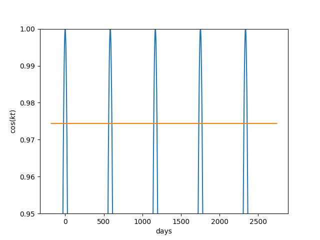
With these constants we can now plot cos(kt) and see when it equals c.

This shows there are five times over the course of eight years when Venus is in apparent retrograde motion.

If we set time t = 0 to be a time when Earth and Venus are aligned, we start in the middle of retrograde period. Venus enters prograde motion 21 days later, and the next retrograde period begins at day 563. So out of every 584 days, Venus spends 42 days in retrograde motion and 542 days in prograde motion.

Related posts

[1] Planets do not exactly orbit in circles. They don’t exactly orbit in ellipses either. Modeling orbits as ellipses is much more accurate than modeling orbits as circles, but not still not perfectly accurate.

[2] 100 Great Problems of Elementary Mathematics: Their History and Solution. By Heinrich Dörrie. Dover, 1965.

[3] There’s nothing unique about observing planets from Earth. Here “Earth” simply means the planet you’re viewing from.

Do incremental improvements add, multiply, or something else?

Suppose you make an x% improvement followed by a y% improvement. Together do they make an (x + y)% improvement? Maybe.

The business principle of kaizen, based on the Japanese 改善 for improvement, is based on the assumption that incremental improvements accumulate. But quantifying how improvements accumulate takes some care.

Add or multiply?

Two successive 1% improvements amount to a 2% improvement. But two successive 50% improvements amount to a 125% improvement. So sometimes you can add, and sometimes you cannot. What’s going on?

An x% improvement multiplies something by 1 + x/100. For example, if you earn 5% interest on a principle of P dollars, you now have 1.05 P dollars.

So an x% improvement followed by a y% improvement multiplies by

(1 + x/100)(1 + y/100) = 1 + (x + y)/100 + xy/10000.

If x and y are small, then xy/10000 is negligible. But if x and y are large, the product term may not be negligible, depending on context. I go into this further in this post: Small probabilities add, big ones don’t.

Interactions

Now let’s look at a variation. Suppose doing one thing by itself brings an x% improvement and doing another thing by itself makes a y% improvement. How much improvement could you expect from doing both?

For example, suppose you find through A/B testing that changing the font on a page increases conversions by 10%. And you find in a separate A/B test that changing an image on the page increases conversions by 15%. If you change the font and the image, would you expect a 25% increase in conversions?

The issue here is not so much whether it is appropriate to add percentages. Since

1.1 × 1.15 = 1.265

you don’t get a much different answer whether you multiply or add. But maybe you could change the font and the image and conversions increase 12%. Maybe either change alone creates a better impression, but together they don’t make a better impression than doing one of the changes. Or maybe the new font and the new image clash somehow and doing both changes together lowers conversions.

The statistical term for what’s going on is interaction effects. A sequence of small improvements creates an additive effect if the improvements are independent. But the effects could be dependent, in which case the whole is less than the sum of the parts. This is typical. Assuming that improvements are independent is often overly optimistic. But sometimes you run into a synergistic effect and the whole is greater than the sum of the parts.

Sequential testing

In the example above, we imagine testing the effect of a font change and an image change separately. What if we first changed the font, then with the new font tested the image? That’s better. If there were a clash between the new font and the new image we’d know it.

But we’re missing something here. If we had tested the image first and then tested the new font with the new image, we might have gotten different results. In general, the order of sequential testing matters.

Factorial testing

If you have a small number of things to test, you can discover interaction effects by doing a factorial design, either a full factorial design or a fractional factorial design.

If you have a large number of things to test, you’ll have to do some sort of sequential testing. Maybe you do some combination of sequential and factorial testing, guided by which effects you have reason to believe will be approximately independent.

In practice, a testing plan needs to balance simplicity and statistical power. Sequentially testing one option at a time is simple, and may be fine if interaction effects are small. But if interaction effects are large, sequential testing may be leaving money on the table.

Help with testing

If you’d like some help with testing, or with web analytics more generally, we can help.

LET’S TALK

The Clausen function

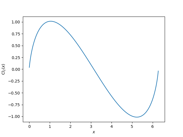
I ran across the Clausen function the other day, and when I saw a plot of the function my first thought was that it looks sorta like a sawtooth wave.

Plot of Clausen function Cl_2

I wondered whether it also sounds like a sawtooth wave, and indeed it does. More on that shortly.

The Clausen function can be defined in terms of its Fourier series:

\text{Cl}_2(x) = \sum_{k=1}^\infty \frac{\sin(kx)}{k^2}

The function commonly known as the Clausen function is one of a family of functions, hence the subscript 2. The Clausen functions for all non-negative integers n are defined by replacing 2 with n on both sides of the defining equation.

The Fourier coefficients decay quadratically, as do those of a triangle wave or sawtooth wave, as discussed here. This implies the function Cl2(x) cannot have a continuous derivative. In fact, the derivative of Cl2(x) is infinite at 0. This follows quickly from the integral representation of the function.

\text{Cl}_2(x)=-\int_0^x\log \left|2\sin\frac{t}{2} \right|\, dt

The fundamental theorem of calculus shows that the derivative

\text{Cl}'_2(x)=-\log \left|2\sin\frac{x}{2} \right|

blows up at 0.

Now suppose we create an audio clip of Cl2(440x). This creates a sound with pitch A 440, but rather than a sinewave it has an unpleasant buzzing sound, much like a sawtooth wave.

clausen2.wav


The harshness of the sound is due to the slow decay of the Fourier coefficients; the Fourier coefficients of more pleasant musical sounds decay much faster than quadratically.

Related posts

Limit of a doodle

Suppose you’re in a boring meeting and you start doodling. You draw a circle, and then you draw a triangle on the outside of that circle.

Next you draw a circle through the vertices of the triangle, and draw a square outside that.

Then you draw a circle through the vertices of the square, and draw a pentagon outside that.

Then you think “Will this ever stop?!”, meaning the meeting, but you could ask a similar question about your doodling: does your sequence of doodles converge to a circle of finite radius, or do they grow without bound?

An n-gon circumscribed on the outside of a circle of radius r is inscribed in a circle of radius

\frac{r}{\cos(\pi/n)}

So if you start with a unit circle, the radius of the circle through the vertices of the N-gon is

\prod_{n=3}^N \frac{1}{\cos(\pi/n)}

and the limit as N → ∞ exists. The limit is known as the polygon circumscribing constant, and it equals 8.7000366252….

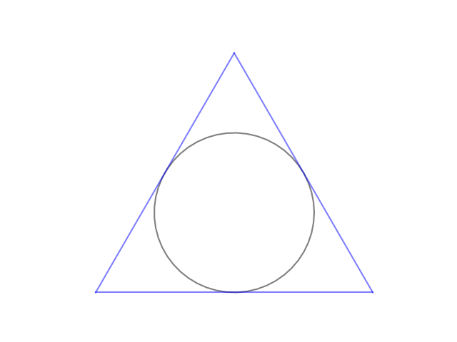
We can visualize the limit by making a plot with large N. The plot is less cluttered if we leave out the circles and just show the polygons. N = 30 in the plot below.

The reciprocal of the polygon circumscribing constant is known as the Kepler-Bouwkamp constant. The Kepler-Bouwkamp constant is the limiting radius if you were to reverse the process above, inscribing polygons at each step rather than circumscribing them. It would make sense to call the Kepler-Bouwkamp constant the polygon inscribing constant, but for historical reasons it is named after Johannes Kepler and Christoffel Bouwkamp.

National Provider Identifier (NPI) and its checksum

Healthcare providers in the United States are required to have an ID number known as the NPI (National Provider Identifier). This is a 10-digit unique identifier which serves as the primary key in a publicly available database. You can use the NPI number to look up a provider’s name, credentials, their practice location, etc. The use of NPI numbers was required by HIPAA.

The specification for the NPI number format says that the first digit must be either 1 or 2. Currently every NPI in the database starts with 1. There are about 8.4 million NPIs currently, so it’ll be a while before they’ll need to roll the first digit over to 2.

The last digit of the NPI is a check sum. The check sum uses the Luhn algorithm, the same check sum used for credit cards and other kinds of identifiers. The Luhn algorithm was developed in 1954 and was designed to be easy to implement by hand. It’s kind of a quirky algorithm, but it will catch all single-digit errors and nearly all transposition errors.

The Luhn algorithm is not applied to the NPI itself but by first prepending 80840 to the (first nine digits of) the NPI.

For example, let’s look at 1993999998. This is not (currently) anyone’s NPI, but it has a valid NPI format because the Luhn checksum of 80840199399999 is 8. We will verify this with the code below.

Python code for Luhn checksum

The following code computes the Luhn checksum.

    def checksum(payload):
        digits = [int(c) for c in reversed(str(payload))]
        s = 0
        for i, d in enumerate(digits):
            if i % 2 == 0:
                t = 2*d
                if t > 9:
                    t -= 9
                s += t
            else:
                s += d
        return (s*9) % 10

And the following checks whether the last digit of a number is the checksum of the previous digits.

    def verify(fullnumber):
        payload = fullnumber // 10
        return checksum(payload) == fullnumber % 10

And finally, the following validates an NPI number.

    def verify_npi(npi):
        return verify(int("80840" + str(npi)))

Here we apply the code above to the hypothetical NPI number mentioned above.

    assert(checksum(80840199399999) == 8)
    assert(verify(808401993999998))
    assert(verify_npi(1993999998))

Related posts

Getting some (algorithmic) SAT-isfaction

How can you possibly solve a mission-critical problem with millions of variables—when the worst-case computational complexity of every known algorithm for that problem is exponential in the number of variables?

SAT (Satisfiability) solvers have seen dramatic orders-of-magnitude performance gains for many problems through algorithmic improvements over the last couple of decades or so. The SAT problem—finding an assignment of Boolean variables that makes a given Boolean expression true—represents the archetypal NP-complete problem and in the general case is intractable.

However, for many practical problems, solutions can be found very efficiently by use of modern methods. This “killer app” of computer science, as described by Donald Knuth, has applications to many areas, including software verification, electronic design automation, artificial intelligence, bioinformatics, and planning and scheduling.

Its uses are surprising and diverse, from running billion dollar auctions to solving graph coloring problems to computing solutions to Sudoku puzzles. As an example, I’ve included a toy code below that uses SMT, a relative of SAT, to find the English language suffix rule for regular past tense verbs (“-ed”) from data.

When used as a machine learning method, SAT solvers are quite different from other methods such as neural networks. SAT solvers can for some problems have long or unpredictable runtimes (though MAXSAT can sometimes relax this restriction), whereas neural networks have essentially fixed inference cost (though looping agent-based models do not).

On the other hand, answers from SAT solvers are always guaranteed correct, and the process is interpretable; this is currently not so for neural network-based large language models.

To understand better how to think about this difference in method capabilities, we can take a lesson from the computational science community. There, it is common to have a well-stocked computational toolbox of both slow, accurate methods and fast, approximate methods.

In computational chemistry, ab initio methods can give highly accurate results by solving Schrödinger’s equation directly, but only scale to limited numbers of atoms. Molecular dynamics (MD), however, relies more on approximations, but scales efficiently to many more atoms. Both are useful in different contexts. In fact, the two methodologies can cross-pollenate, for example when ab initio calculations are used to devise force fields for MD simulations.

A lesson to take from this is, it is paramount to find the best tool for the given problem, using any and all means at one’s disposal.

The following are some of my favorite general references on SAT solvers:

It would seem that unless P = NP, commonly suspected to be false, the solution of these kinds of problems for any possible input is hopelessly beyond reach of even the world’s fastest computers. Thankfully, many of the problems we care about have an internal structure that makes them much more solvable (and likewise for neural networks). Continued improvement of SAT/SMT methods, in theory and implementation, will greatly benefit the effective solution of these problems.

A toy example: find the English past tense suffix rule using Z3

import csv
import z3

def char2int(c): return ord(c) - ord('a')

def int2char(i): return chr(i + ord('a'))

# Access the language data from the file.
with open('eng_cols.txt', newline='') as csvfile:
    reader = csv.reader(csvfile, delimiter='\t')
    table = [row for row in reader]

nrow, ncol = len(table), len(table[0])

# Identify which columns of input table have stem and targeted word form.
stem_col, form_col = 0, 1

# Calculate word lengths.
nstem = [len(table[i][stem_col]) for i in range(nrow)]
nform = [len(table[i][form_col]) for i in range(nrow)]

# Length of suffix being sought.
ns = 2

# Initialize optimizer.
solver = z3.Optimize()

# Define variables to identify the characters of suffix; add constraints.
var_suf = [z3.Int(f'var_suf_{i}') for i in range(ns)]

for i in range(ns):
    solver.add(z3.And(var_suf[i] >= 0, var_suf[i] < 26))

# Define variables to indicate whether the given word matches the rule.
var_m = [z3.Bool(f'var_m_{i}') for i in range(nrow)]

# Loop over words.
for i in range(nrow):

    # Constraint on number of characters.
    constraints = [nform[i] == nstem[i] + ns]

    # Constraint that the form contains the stem.
    for j in range(nstem[i]):
        constraints.append(
            table[i][stem_col][j] == table[i][form_col][j]
                if j < nform[i] else False)

    # Constraint that the end of the word form matches the suffix. 
    for j in range(ns):
        constraints.append(
            char2int(table[i][form_col][nform[i]-1-j]) == var_suf[j]
                if j < nform[i] else False)

    # var_m[i] is the "and" of all these constraints.
    solver.add(var_m[i] == z3.And(constraints))

# Seek suffix that maximizes number of matches.
count = z3.Sum([z3.If(var_m[i], 1, 0) for i in range(nrow)])
solver.maximize(count)

# Run solver, output results.
if solver.check() == z3.sat:
    model = solver.model()
    suf = [model[var_suf[i]] for i in range(ns)]
    print('Suffix identified: ' +
          ''.join(list([int2char(suf[i].as_long())
                        for i in range(ns)]))[::-1])
    print('Number of matches: ' + str(model.evaluate(count)) +
          ' out of ' + str(nrow) + '.')

    var_m_values = [model[var_m[i]] for i in range(nrow)]

    print('Matches:')
    for i in range(nrow):
        if var_m_values[i]:
            print(table[i][stem_col], table[i][form_col])

Computing Γ(z) for complex z with tables

In the previous post I mentioned that the general strategy for computing a mathematical function using tables is to first reduce the function argument to be within the range of the tabulated values, and then to use interpolation to compute the function at values that are not directly tabulated.

The second step is always the same, applying Lagrange interpolation with enough points to get the accuracy you need. But the first step, range reduction, depends on the function being evaluated. And as the previous post concluded, evaluating more advanced functions generally requires more advanced range reduction.

Real argument

For the gamma function, the identity

\Gamma(x + 1) = x\, \Gamma(x)

can be used to reduce the problem of computing Γ(x) for any real x to the problem of computing Γ(x) for x in the interval [1, 2]. If x is large, the identity will have to be applied many times and so this would be a lot of work. However, the larger x is, the more accurate Stirling’s approximation becomes.

Complex argument

Computing Γ(x + iy) is more complex, pardon the pun. We can still use the identity above to reduce the real part x of the argument to lie in the interval [1, 2], but what about the complex part y?

Abramowitz and Stegun, Table 6.7, tabulates the principal branch of log Γ(x + iy) for x from 1 to 2 and for y from 0 to 10, both in increments of 0.1. Generally the logarithm of the gamma function is more useful in computation than the gamma function itself. It is also easier to interpolate, which I imagine is the main reason A&S tabulate it rather than the gamma function per se. A note below Table 6.7 says that linear interpolation gives about 3 significant figures, and eight-point interpolation gives about 8 figures.

By the Schwarz reflection principle,

\Gamma(\bar{z}) = \overline{\Gamma(z)}

and with this we can extend our range on y to [−10, 10].

Large imaginary part

What about larger y? We have two options: the duplication formula and Stirling’s approximation.

The duplication formula

\Gamma(2z) = \frac{1}{\sqrt{2\pi}}2^{2z - \frac{1}{2}} \Gamma(z) \Gamma\left(z + \tfrac{1}{2} \right )

lets us compute Γ(2z) if we can compute Γ(z) and Γ(z + ½).

Stirling’s approximation for Γ(z) is accurate when |z| is large, and |x + iy| is large when |y| is large.

More posts on using tables

Calculating trig functions from tables

It takes some skill to use tables of mathematical functions; it’s not quite as simple as it may seem. Although it’s no longer necessary to use tables, it’s interesting to look into the details of how it is done.

For example, the Handbook of Mathematical Functions edited by Abramowitz and Stegun tabulates sines and cosines in increments of one tenth of a degree, from 0 degrees to 45 degrees. What if your angle was outside the range 0° to 45° or if you needed to specify your angle more precisely than 1/10 of a degree? What if you wanted, for example, to calculate cos 203.147°?

The high-level answer is that you would use range reduction and interpolation. You’d first use range reduction to reduce the problem of working with any angle to the problem of working with an angle between 0° and 45°, then you’d use interpolation to get the necessary accuracy for a value within this range.

OK, but how exactly do you do the range reduction and how exactly do you to the interpolation? This isn’t deep, but it’s not trivial either.

Range reduction

Since sine and cosine have a period of 360°, you can add or subtract some multiple of 360° to obtain an angle between −180° and 180°.

Next, you can use parity to reduce the range further. That is, since sin(−x) = −sin(x) and cos(−x) = cos(x) you can reduce the problem to computing the sine or cosine of an angle between 0 and 180°.

The identities sin(180° − x) = sin(x) and cos(180° −x) = −cos(x) let you reduce the range further to between 0 and 90°.

Finally, the identities cos(x) = sin(90° − x) and sin(x) = cos(90° − x) can reduce the range to 0° to 45°.

Interpolation

You can fill in between the tabulated angles using interpolation, but how accurate will your result be? How many interpolation points will you need to use in order to get single precision, e.g. an error on the order of 10−7?

The tables tell you. As explained in this post on using a table of logarithms, the tables have a notation at the bottom of the table that tells you how many Lagrange interpolation points to use and what kind of accuracy you’ll get. Five interpolation points will give you roughly single precision accuracy, and the notation gives you a little more accurate error bound. The post on using log tables also explains how Lagrange interpolation works.

Beyond trig functions

I intend to write more posts on using tables. The general pattern is always range reduction and interpolation, but it takes more advanced math to reduce the range of more advanced functions.

Update: The next post shows how to use tables to compute the gamma function for complex arguments.

Rapidly convergent series for ellipse perimeter

The previous post looked at two simple approximations for the perimeter of an ellipse. Approximations are necessary since the perimeter of an ellipse cannot be expressed as an elementary function of the axes.

Kepler noted in 1609 that you could approximate the perimeter of an ellipse as the perimeter of a circle whose radius is the mean of the semi-axes of the ellipse, where the mean could be either the arithmetic mean or the geometric mean. The previous post showed that the arithmetic mean is more accurate, and that it under-estimates the perimeter. This post will explain both of these facts.

There are several series for calculating the perimeter of an ellipse. In 1798 James Ivory came up with a series that converges more rapidly than previously discovered series. Ivory’s series is

P = \pi (a+b) \left(1 + \sum_{n=1}^\infty \left(\frac{(2n-1)!!}{2^n n!}\right)^2 \frac{h^n}{(2n-1)^2}\right)

where

h = \frac{(a-b)^2}{(a+b)^2}

If you’re not familiar with the !! notation, see this post on multifactorials.

The 0th order approximation using Ivory’s series, dropping all the infinite series terms, corresponds to Kepler’s approximation using the arithmetic mean of the semi-axes a and b. By convention the semi-major axis is labeled a and the semi-minor axis b, but the distinction is unnecessary here since Ivory’s series is symmetric in a and b.

Note that h ≥ 0 and h = 0 only if the ellipse is a circle. So the terms in the series are positive, which explains why Kepler’s approximation under-estimates the perimeter.

Using just one term in Ivory’s series gives a very good approximation

P \approx \pi(a + b)\left(1 + \frac{1}{4} \frac{(a-b)^2}{(a+b)^2}\right)

The approximation error increases as the ratio of a to b increases, but even for a highly eccentric ellipse like the orbit of the Mars Orbital Mission, the ratio of a to b is only 2, and the relative approximation error is about 1/500, about 12 times more accurate than Kepler’s approximation.