When is less data less private?

If I give you a database, I give you every row in the database. So if you delete some rows from the database, you have less information, not more, right?

This seems very simple, and it mostly is, but there are a couple subtleties.

A common measure in data privacy is k-anonymity. The idea is that if at least k individuals in a data set share some set of data values, and k is large enough, then the privacy of those individuals is protected.

Now suppose you randomly select a single record from a database that was deemed deidentified because it satisfied k-anonymity with k = 10. Now your new dataset, consisting of only one record, is k-anonymous with k = 1: every record is unique because there’s only one record. But how is this person’s data any less private that it was before?

Note that I said above that you selected a record at random. If you selected the row using information that you know but which isn’t in the database, you might have implicitly added information. But if you select a subset of data, using only information explicit in that data, you haven’t added information.

Here’s where k-anonymity breaks down. The important measure is k-anonymity in the general population, not k-anonymity in a data set, unless you know that someone is in the data set.

If you find someone named John Cook in a data set, you probably haven’t found my information, even if there is only one person by that name in the data set. My name may or may not be common in that particular data set, but my name is common in general.

The number of times a combination of data fields gives a lower bound on how often the combination appears in general, so k-anonymity in a data set is a good sign for privacy, but the lack of k-anonymity is not necessarily a bad sign. The latter could just be an artifact of having a small data set.

Related posts

How likely is a random variable to be far from its center?

There are many answers to the question in the title: How likely is a random variable to be far from its center?

The answers depend on how much you’re willing to assume about your random variable. The more you can assume, the stronger your conclusion. The answers also depend on what you mean by “center,” such as whether you have in mind the mean or the mode.

Chebyshev’s inequality says that the probability of a random variable X taking on a value more than k standard deviations from its mean is less than 1/k². This of course assumes that X has a mean and a standard deviation.

If we assume further that X is unimodal, and k ≥ √(8/3), then the conclusion of Chebyshev’s inequality can be strengthened to saying that the probability of X being more than k standard deviations from its mean is less than 4/9k². This is the Vysochanskiĭ-Petunin inequality. More on this inequality here.

If k ≤ √(8/3) the Vysochanskiĭ-Petunin inequality says the probability of X being more than k standard deviations from its mean is less than

4/3k² − 1/3.

Gauss’ inequality is similar to the Vysochanskiĭ-Petunin inequality. It also assumes X is unimodal, and for convenience we will assume the mode is at zero (otherwise look at Y = Xm where m is the mode of X). Gauss’ inequality bounds the probability of X being more than k standard deviations away from its mode rather than its mean.

Let τ² be the expected value of X². If the mean value of X is zero then τ² = σ² and the equations below are similar to the Vysochanskiĭ-Petunin inequality. But Gauss does not require that X has mean zero.

Gauss’ inequality says that

P(|X| > kτ) ≤ 4/9k²

if k ≥ √(4/3) and

P(|X| > kτ) ≤ 1 − k/(√3 τ)

otherwise.

Gauss’ inequality is stronger than the Vysochanskiĭ-Petunin inequality when X has zero mean, but it is also assuming more, namely that the mean and mode are equal.

Related post: Strengthening Markov’s inequality with conditional probability.

Two-digit zip codes

It’s common to truncate US zip codes to the first three digits for privacy reasons. Truncating to the first two digits is less common, but occurs in some data sets.

HIPAA Safe Harbor requires sparse 3-digit zip codes to be suppressed; even when rolled up to three digits some regions are still sparsely populated.

How sparse can a two-digit zip code region be? Empty. The population of all zip codes starting with 09 is zero. That’s because all zip codes of the form 09XXX are overseas military bases and not anyone’s permanent residence.

Aside from that, the least populated 2-digit zip code is 69 with a population of about 175,000.

The most populated 2-digit zip code is 33 with a population of about 10,500,000.

So the ratio of the largest population to the smallest non-zero population is about 60.

What if we roll up all the way to 1-digit zip codes? Now things are more evenly distributed. The smallest region is 5 with a population of about 17.5M and the largest is 9 with a population of about 54M. A ratio of about 3.

Related posts

Beta inequality symmetries

I was thinking about the work I did when I worked in biostatistics at MD Anderson. This work was practical rather than mathematically elegant, useful in its time but not of long-term interest. However, one result came out of this work that I would call elegant, and that was a symmetry I found.

Let X be a beta(a, b) random variable and let Y be a beta(c, d) random variable. Let g(a, b, c, d) be the probability that a sample from X is larger than a sample from Y.

g(a, b, c, d) = Prob(X > Y)

This function often appeared in the inner loop of a simulation and so we spent thousands of CPU-hours computing its values. I looked for ways to evaluate this function more quickly, and along the way I found a symmetry.

The function I call g was studied by W. R. Thompson in 1933 [1]. Thompson noted two symmetries:

g(a, b, c, d) = 1 − g(c, d, a, b)

and

g(a, b, c, d) = g(d, c, b, a)

I found an additional symmetry:

g(a, b, c, d) = g(d, b, c, a).

The only reference to this result in a journal article as far as I know is a paper I wrote with Saralees Nadarajah [2]. That paper cites an MD Anderson technical report which is no longer online, but I saved a copy here.

Related posts

[1] W. R. Thompson. On the Likelihood that One Unknown Probability Exceeds Another in View of the Evidence of Two Samples. Biometrika, Volume 25, Issue 4. pp. 285 – 294.

[2] John D. Cook and Saralees Nadarajah. Stochastic Inequality Probabilities for Adaptively Randomized Clinical Trials. Biometrical Journal. 48 (2006) pp 256–365.


The Five Safes data privacy framework

Five safes

The Five Safes decision framework was created a couple decades ago by Felix Ritchie at the UK Office for National Statistics. It is a framework for evaluating the safe use of confidential data, particularly by government agencies. You can find a description of the Five Safes, for example, in NIST SP 800-188.

The Five Safes are

  1. Safe projects
  2. Safe people
  3. Safe settings
  4. Safe data
  5. Safe outputs

Safe projects asks whether the use of the data is appropriate. It doesn’t matter how safe the access controls and so forth are if the project itself is inappropriate.

Safe people asks whether the users be trusted to use the data in an appropriate manner. For health care data, for example, one could ask whether users have had HIPAA training.

Safe settings applies to physical access. Does the facility hosting the data limit unauthorised access?

Safe data asks about statistical disclosure control, whether the data itself poses a disclosure risk. For example, have the data been adequately deidentified?

Safe outputs asks whether the output of the project poses a privacy risk.

Various approaches to data privacy have different trade-offs between the Five Safes. Differential privacy focuses on safe outputs. There are mathematical guarantees that the outputs satisfy a certain definition of privacy. The data itself is regarded as unsafe, and so it is important that the people and settings are safe.

HIPAA expert determination focuses on safe data. Often there is a sort of firewall with data considered safe on one side for one set of reasons (patient consent, a BAA contract, etc.) and considered safe on the other side of the wall because the data itself is safe, i.e. properly deidentified.

Safe Harbor is unrelated to the Five Safes. Safe Harbor is a provision under the HIPAA Privacy Rule for deeming certain data safe. Whether the Safe Harbor rules actually result in safe data depends on context. Data may comply with the letter of the law appealing to Safe Harbor, and yet not protect individuals in the data from being identified.

If you would like help evaluating the privacy aspects of a data analysis project, let’s talk.

Database reconstruction attacks

In 2018, three researchers from the US Census Bureau published a paper entitled “Understanding Database Reconstruction Attacks on Public Data.” [1] The article showed that private data on many individuals could be reverse engineered from public data.

As I wrote about a few days ago, census blocks are at the bottom of the US Census Bureau’s hierarchy of geographical entities. On average a census block may contain about 40 people, but a block may contain only one person.

In hindsight it seems fairly obvious that data reported at the census block level is vulnerable to re-identification, and yet this doesn’t seem to have been noticed before around 2000. There were some privacy measures in place before then, but it wasn’t clear that these methods were insufficient to protect privacy.

You can think of each fact about each person as a variable and each reported statistic as an equation. When the number of equations is comparable to the number of variables, it’s possible that the system of equations has a unique solution. (We know a priori that there exists at least one solution, assuming the reported statistics were correctly computed.)

It’s not quite as simple as that, though that is roughly the idea in [1]. The data collected in the census is binary or integer data, which makes database reconstruction easier. Ages, for example, are integers, and typically integers less than 100.

One of the techniques the Census Bureau previously used in an attempt to protect individual privacy was a sort of small cell rule, a rule to not report statistics based on three or fewer individuals. This may or may not help. In the example given in [1], there are 7 people in a hypothetical census block, of whom 4 are adults and an unreported number are minors. Determining the number of minors is left as an exercise for the reader.

The set of equations is more complicated than a set of linear equations. The inference problem is a matter of logic programming or constraint satisfaction. Missing data is not always as trivial to reconstruct as in the preceding paragraph, but missing data can still convey partial information. The very fact that the data is missing tells you something.

The discrete nature of the data makes the solution process both harder and easier. It makes things harder in the sense of requiring a more complicated solution algorithm, but it makes things easier in the sense of increasing the likelihood that the equations have a unique solution.

This is why the Census Bureau embraced differential privacy for the 2020 census. They had no choice but to do something substantially different than they had done in the past once it became apparent that their previous approach failed rather badly at protecting confidentiality.

Related posts

[1] Simson Garfinkel, John M. Abowd, Christain Martindale. Understanding Database Reconstruction Attacks on Public Data. ACM Quque, October 2018. The article was also published in Communications of the ACM in March 2019.

Differentially private stochastic gradient descent

Let’s work our way up to differentially private stochastic gradient descent (DP-SGD) a little at a time. We’ll first look at gradient descent, then stochastic gradient descent, then finally differentially private stochastic gradient descent.

Gradient descent

We’ll start with gradient descent. Suppose you have a function of several variables f(x) where x is a vector. Then the gradient ∇f(x) points in the direction of greatest increase in f, and its negative −∇f(x) points in the direction of greatest decrease. So you can decrease the function f by moving in the direction −∇f(x). You can turn this observation into an algorithm for minimizing f. Find the gradient, take a step in the opposite direction. Rinse, lather, and repeat. The gradient descent method is also called steepest descent because locally you’re always moving in the direction of steepest descent.

Locally is the key word here. In some finite neighborhood of x, −∇f(x) points in a direction that will decrease the value of f. How large is this neighborhood? Hard to say. How long a step should you take? Also hard to say.

If your function f is strictly convex, then there is a global minimum, and the gradient descent algorithm will converge to it.

Stochastic gradient descent

What could go wrong? If your objective function f is strictly convex, convergence is guaranteed, but convergence may be slow. The method is always locally optimal, but optimal may mean inside a tiny little neighborhood of where you start each iteration.

Gradient descent can meander through a valley, a nearly flat spot of the objective function, taking tiny steps back and forth and not making much progress toward finding the low point.

Another problem is that gradient descent can get stuck in a local minimum. If f is strictly convex then there are no local minima, just one global minimum, but stochastic gradient descent is used to minimize functions that are not convex and that may have many local minima.

So to get unstuck, either from being stuck at a local minimum or from a flat spot, stochastic gradient descent adds randomness.

The objective functions used in training neural networks have many variables, maybe millions or billions, and these functions are far from convex.

Differentially private stochastic gradient descent

Now suppose you’re doing machine learning on sensitive data, such as medical records. You want to train a model on the data, but you don’t want the model to memorize and leak personally identifiable information (PII) or protected health information (PHI).

If you were simply querying the data, rather than training a network on it, you could apply differential privacy to queries, adding an amount of noise to each query result calibrated to be just enough randomness to preserve privacy. But training a neural network is far more complicated that running a SQL query.

The core idea of differential privacy is that any individual’s presence or absence from a database must not make much difference, in a rigorously quantified sense. Any outcome that happened with someone in the database could plausibly have happened without that person being in the database. Stochastic gradient descent is already a randomized algorithm, and variations on the algorithm can also provide differential privacy guarantees. See [1] for a seminal paper and [2] for a later refinement.

Related posts

[1] Shuang Song, Kamalika Chaudhuri, Anand D. Sarwate. Stochastic gradient descent with differentially private updates. 2013 IEEE Global Conference on Signal and Information Processing (GlobalSIP)

[2] Abadi et al. Deep Learning with Differential Privacy. arXiv:1607.00133 [stat.ML]

Using classical statistics to avoid regulatory burden

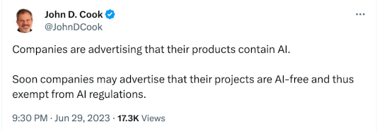
On June 29 this year I said on Twitter that companies would start avoiding AI to avoid regulation.

Companies are advertising that their products contain AI. Soon companies may advertise that their projects are AI-free and thus exempt from AI regulations.

I followed that up with an article Three advantages of non-AI models. The third advantage I listed was

Statistical models are not subject to legislation hastily written in response to recent improvements in AI. The chances that such legislation will have unintended consequences are roughly 100%.

Fast forward four months and we now have a long, highly-detailed executive order, Executive Order 14110, effecting all things related to artificial intelligence. Here’s an excerpt:

… the Secretary [of Commerce] shall require compliance with these reporting requirements for: any model that was trained using a quantity of computing power greater than 1026 integer or floating-point operations, or using primarily biological sequence data and using a quantity of computing power greater than 1023 integer or floating-point operations; and any computing cluster that has a set of machines physically co-located in a single datacenter, transitively connected by data center networking of over 100 Gbit/s, and having a theoretical maximum computing capacity of 1020 integer or floating-point operations per second for training AI.

If a classical model can do what you need, you are not subject to any regulations that will flow out of the executive order above, not if these regulations use definitions similar to those in the executive order.

How many floating point operations does it take to train, say, a logistic regression model? It depends on the complexity of the model and the amount of data fed into the model, but it’s not 1020 flops.

Can you replace an AI model with something more classical like a logistic regression model or a Bayesian hierarchical model? Very often. I wouldn’t try to compete with Midjourney for image generation that way, but classical models can work very well on many problems. These models are much simpler—maybe a dozen parameters rather than a billion parameters—and so are much better understood (and so there is less fear of such models that leads to regulation).

I had a client that was using some complicated models to predict biological outcomes. I replaced their previous models with a classical logistic regression model and got better results. The company was so impressed with the improvement that they filed a patent on my model.

If you’d like to discuss whether I could help your company replace a complicated AI model with a simpler statistical model, let’s talk.

Identifiers depend on context

Can you tell who someone is from their telephone number? That’s kinda the point of telephone numbers, to let you contact someone. And indeed telephone number is one the 18 identifiers under HIPAA Safe Harbor.

But whether any piece of information allows you to identify someone depends on context. If you don’t have access to a phone, or a phone book, or any electronic counterpart of a phone book, then a phone number doesn’t allow you to identify anyone. But once you can call a phone number or enter it into a search engine, then the phone number is identifiable. Maybe.

What if the number belongs to a burner phone? Then it would be harder to learn the identity of the person who owns the number, but not impossible. Maybe you couldn’t learn anything about the owner, but law enforcement officials could. Again identifiability depends on context.

An obvious identifier like a phone number might not be an identifier in some special circumstance. And an apparently useless bit of information might reveal someone’s identity in another circumstance.

HIPAA’s Safe Harbor Rule tries to say apart from context what kinds of data are identifiable. But if you read the Safe Harbor Rule carefully you’ll notice it isn’t so context-free as it seems. The last item in the list of 18 items to remove is “any other unique identifying number, characteristic, or code.” What might be an identifying characteristic? That depends on context.

V-statistics

A few days ago I wrote about U-statistics, statistics which can be expressed as the average of a symmetric function over all combinations of elements of a set. V-statistics can be written as an average of over all products of elements of a set.

Let S be a statistical sample of size n and let h be a symmetric function of r elements. The average of h over all subsets of S with r elements is a U-statistic. The average of h over the Cartesian product of S with itself r times

\underbrace{S \times S \times \cdots \times S}_{n \text{ times}}

is a V-statistic.

As in the previous post, let h(x, y) = (xy)²/2. We can illustrate the V-statistic associated with h with Python code as before.

    import numpy as np
    from itertools import product

    def var(xs):
        n = len(xs)
        h = lambda x, y: (x - y)**2/2
        return sum(h(*c) for c in product(xs, repeat=2)) / n**2

    xs = np.array([2, 3, 5, 7, 11])
    print(np.var(xs))
    print(var(xs))

This time, however, we iterate over product rather than over combinations. Note also that at the bottom of the code we print

   np.var(xs)

rather than

   np.var(xs, ddof=1)

This means our code here is computing the population variance, not the sample variance. We could make this more explicit by supplying the default value of ddof.

   np.var(xs, ddof=0)

The point of V-statistics is not to calculate them as above, but that they could be calculated as above. Knowing that a statistic is an average of a symmetric function is theoretically advantageous, but computing a statistic this way would be inefficient.

U-statistics are averages of a function h over all subsamples of S of size r without replacement. V-statistics are averages of h over all subsamples of size r with replacement. The difference between sampling with or without replacement goes away as n increases, and so V-statistics have the same asymptotic properties as U-statistics.

Related posts