The date of Easter
The church fixed Easter to be the first Sunday after the first full moon after the Spring equinox. They were choosing a date in the Roman (Julian) calendar to commemorate an event whose date was known according to the Jewish lunisolar calendar, hence the reference to equinoxes and full moons.
The previous post explained why the Eastern and Western dates of Easter differ. The primary reason is that both churches use March 21 as the first day of Spring, but the Eastern church uses March 21 on the Julian calendar and the Western church uses March 21 on the Gregorian calendar.
But that’s not the only difference. The churches chose different algorithms for calculating when the first full moon would be. The date of Easter doesn’t depend on the date of the full moon per se, but the methods used to predict full moons.
This post will show why determining the date of the full moon is messy.
Lunation length
The moon takes between 29 and 30 days between full moons (or between new moons, which are easier to objectively measure). This period is called a lunation. The average length of a lunation is L = 29.530588853 days. This is not a convenient number to work with, and so there’s no simple way of reconciling the orbital period of the moon with the rotation period of the earth [1]. Lunar calendars alternate months with 29 and 30 days, but they can’t be very accurate, so they have to have some fudge factor analogous to leap years.
The value of L was known from ancient times. Meton of Athens calculated in 432 BC that 235 lunar cycles equaled 19 tropical years or 6940 days. This corresponds to L ≈ 29.5319. Around a century later the Greek scholar Callippus refined this to 940 cycles in 76 years or 27,759 days. This corresponds to L ≈ 29.53085.
The problem wasn’t knowing L but devising a convenient way of working with L. There is no way to work with lunations that is as easy as the way the Julian (or even the more complicated Gregorian) calendar reconciles days with years.
Approximations
Let’s look at the accuracy of several approximations for L. We’d like an approximation that is not only accurate in an absolute sense, but also accurate relative to its complexity. The complexity of a fraction is measured by a height function. We’ll use what’s called the “classic” height function: log( max(n, d) ) where n and d are the numerator and denominator of a fraction. Since we’re approximating a number bigger than 1, this will be simply log(n).
We will compare the first five convergents, approximations that come from the continued fraction form of L, and the approximations of Meton and Callippus. Here’s a plot.
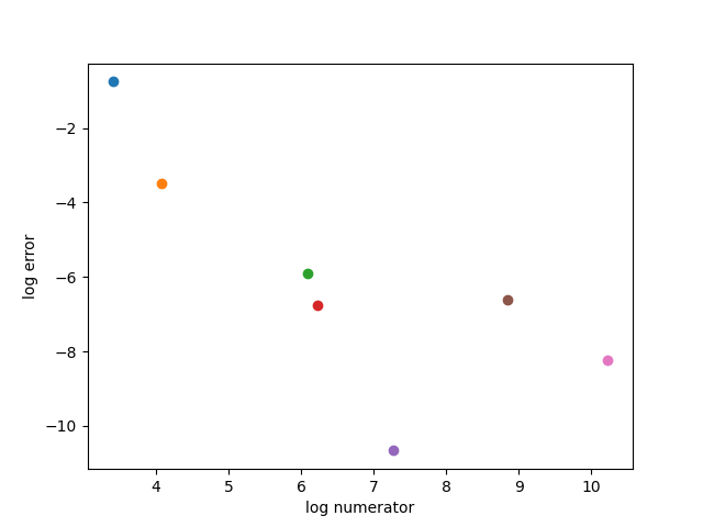
And here’s the code that produced the plot, showing the fractions used.
from numpy import log
import matplotlib.pyplot as plt

fracs = [
    (30, 1),
    (59, 2),
    (443, 15),
    (502, 17),
    (1447, 49),
    (6940, 235),
    (27759, 940)
]

def error(n, d):
    L = 29.530588853
    return abs(n/d - L)

for f in fracs:
    plt.plot(log(f[0]), log(error(*f)), 'o')
plt.xlabel("log numerator")
plt.ylabel("log error")
plt.show()
The approximation 1447/49 is the best by far, both in absolute terms and relative to the size of the numerator. But it’s not very useful for calendar design because 1447 is not nicely related to the number of days in a year.
[1] The time between full moons is a synodic month, the time it takes for the moon to return to the same position relative to the sun. This is longer than a sidereal month, the time it takes the moon to complete one orbit relative to the fixed stars.