The multiplication table of a finite group forms a Latin square.
You form the multiplication table of a finite group just as you would the multiplication tables from your childhood: list the elements along the top and side of a grid and fill in each square with the products. In the context of group theory the multiplication table is called a Cayley table.
There are two differences between Cayley tables and the multiplication tables of elementary school. First, Cayley tables are complete because you can include all the elements of the group in the table. Elementary school multiplication tables are the upper left corner of an infinite Cayley table for the positive integers.
(The positive integers do not form a group under multiplication because only 1 has a multiplicative inverse. The positive integers form a magma, not a group, but we can still talk of the Cayley table of a magma.)
The other difference is that the elements of a finite group typically do not have a natural order, unlike integers. It’s conventional to start with the group identity, but other than that the order of the elements along the top and sides could be arbitrary. Two people may create different Cayley tables for the same group by listing the elements in a different order.
A Cayley table is necessarily a Latin square. That is, each element appears exactly once in each row and column. Here’s a quick proof. The row corresponding to the element a consists of a multiplied by each of the elements of the group. If two elements were the same, i.e. ab = ac for some b and c, then b = c because you can multiply on the left by the inverse of a. Each row is a permutation of the group elements. The analogous argument holds for columns, multiplying on the right.
Not all Latin squares correspond to the Cayley table of a group. Also, the Cayley table of an algebraic structure without inverses may not form a Latin square. The Cayley table for the positive integers, for example, is not a Latin square.
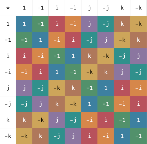
Here’s an example, the Cayley table for Q8, the group of unit quaternions. The elements are ±1, ±i, ±j, and ±k and the multiplication is the usual multiplication for quaternions:
i² = j² = k² = ijk = −1.
as William Rowan Hamilton famously carved into the stone of Brougham Bridge. I colored the cells of the table to make it easier to scan to verify that table is a Latin square.