Zooming in on a fractalish plot

The exponential sum of the day page on my site draws an image every day by plugging the month, day, and year into a formula. Details here.

Today’s image looks almost solid blue in the middle.

The default plotting line width works well for most days. For example, see what the sum of the day will look line on July 1 this year. Making the line width six times thinner reveals more of the detail in the middle.

You can see even more detail in a PDF of the plot.

Most ints are not floats

All integers are real numbers, but most computer representations of integers do not equal computer representations of real numbers.

To make the statement above precise, we have to be more specific about what we mean by computer integers and floating point numbers. I’ll use int32 and int64 to refer to 32-bit and 64-bit signed integers. I’ll use float32 and float64 to refer to IEEE 754 single precision and double precision numbers, what C calls float and double.

Most int32 numbers cannot be represented exactly by a float32. All int32 numbers can be represented approximately as float32 numbers, but usually not exactly. The previous statements remain true if you replace “32” everywhere by “64.”

32 bit details

The int32 data type represents integers −231 through 231 − 1. The float32 data type represents numbers of the form

± 1.f × 2e

where 1 bit represents the sign, 23 bits represent f, and 8 bits represent e.

The number n = 224 can be represented by setting the fractional part f  to 0 and setting the exponent e to 24. But the number n + 1 cannot be represented as a float32 because its last bit would fall off the end of f:

224 + 1 = (1 + 2−24) 224 = 1.000000000000000000000001two × 224

The bits in f fill up representing the 23 zeros after the decimal place. There’s no 24th bit to store the final 1.

For each value of e, there are 223 possible values of f. So for each of e = 24, 25, 26, …, 31 there are 223 representable integers, for a total of 8 × 223.

So of the 231 non-negative integers that can be represented by an int32 data type, only 9 × 223 can also be represented exactly as a float32 data type. This means about 3.5% of 32-bit integers can be represented exactly by a 32-bit float.

64 bit details

The calculations for 64-bit integers and 64-bit floating point numbers are analogous. Numbers represented by float64 data types have the form

± 1.f × 2e

where now f has 52 bits and e has 11.

Of the 263 non-negative integers that can be represented by an int64 data type, only 11 × 252 can also be represented exactly as a float64 data type. This means about 0.5% of 64-bit integers can be represented exactly by a 64-bit float.

A note on Python

Python’s integers have unlimited range, while its floating point numbers correspond to float64. So there are two reasons an integer might not be representable as a float: it may be larger than the largest float, or it may require more than 53 bits of precision.

Related posts

Test whether a large integer is a square

Years ago I wrote about a fast way to test whether an integer n is a square. The algorithm rules out a few numbers that cannot be squares based on their last (hexidecimal) digit. If the the integer passes through this initial screening, the algorithm takes the square root of n as a floating point number, rounds  to an integer, and tests whether the square of the rest equals n.

What’s wrong with the old algorithm

The algorithm described above works fine if n is not too large. However, it implicitly assumes that the integer can be represented exactly as a floating point number. This is two assumptions: (1) it’s not too large to represent, and (2) the representation is exact.

A standard 64-bit floating point number has 1 bit for the sign, 11 bits for the exponent, and 52 bits for the significand. (More on that here.) Numbers will overflow if they run out of exponent bits, and they’ll lose precision if they run out of significand bits. So, for example, 21024 will overflow [1]. And although 253 + 1 will not overflow, it cannot be represented exactly.

These are illustrated in Python below.

    >>> float(2**1024)
    OverflowError: int too large to convert to float
    >>> n = 2**53
    >>> float(n) == float(n + 1)
    True

A better algorithm

The following algorithm [2] uses only integer operations, and so it will work exactly for arbitrarily large integers in Python. It’s a discrete analog of Newton’s square root algorithm.

    def intsqrt(N):
        n = N
        while n**2 > N:
            n = (n + N//n) // 2
        return n

    def issquare(N):
        n = intsqrt(N)
        return n**2 == N

The function issquare will test whether N is a square. The function intsqrt is broken out as a separate function because it is independently useful since it returns ⌊√N⌋.

The code above correctly handles examples that the original algorithm could not.

    >>> issquare(2**1024)
    True
    >>> issquare(2**54)
    True
    >>> issquare(2**54 + 1)
    False

You could speed up issquare by quickly returning False for numbers that cannot be squared on account of their final digits (in some base—maybe you’d like to use a base larger than 16) as in the original post.

[1] The largest allowed exponent is 1023 for reasons explained here.

[2] Bob Johnson. A Route to Roots. The Mathematical Gazette, Vol. 74, No. 469 (Oct., 1990), pp. 284–285

Legendre and Ethereum

What does an eighteenth century French mathematician have to do with the Ethereum cryptocurrency?

A pseudorandom number generator based on Legendre symbols, known as Legendre PRF, has been proposed as part of a zero knowledge proof mechanism to demonstrate proof of custody in Ethereum 2.0. I’ll explain what each of these terms mean and include some Python code.

The equation x² = a mod p is solvable for some values of a and not for others. The Legendre symbol

\left(\frac{a}{p}\right)

is defined to be 1 if a has a square root mod p, and −1 if it does not. Here a is a positive integer and p is a (large) prime [1]. Note that this is not a fraction, though it looks like one.

As a varies, the Legendre symbols vary randomly. Not literally randomly, of course, but the act random enough to be useful as a a pseudorandom number generator.

Legendre PRF

Generating bits by computing Legendre symbols is a lot more work than generating bits using a typical PRNG, so what makes the Legendre PRF of interest to Ethereum?

Legendre symbols can be computed fairly efficiently. You wouldn’t want to use the Legendre PRF to generate billions of random numbers for some numerical integration computation, but for a zero knowledge proof you only need to generate a few dozen bits.

To prove that you know a key k, you can generate a string of pseudorandom bits that depend on the key. If you can do this for a few dozen bits, it’s far more likely that you know the key than that you have guessed the bits correctly. Given k, the Legendre PRF computes

L_k(x) = \frac{1}{2}\left( 1 - \left( \frac{k+x}{p}\right) \right)

for n consecutive values of x [2].

One reason this function is of interest is that it naturally lends itself to multiparty computation (MPC). The various parties could divide up the range of x values that each will compute.

The Legendre PRF has not been accepted to be part of Ethereum 2.o. It’s only been proposed, and there is active research into whether it is secure enough.

Python code

Here’s a little Python scrypt to demonstrate using Lk(x).

    from sympy import legendre_symbol

    def L(x, k, p):
        return (1 - legendre_symbol(x + k, p)) // 2

    k = 20250626
    p = 2**521 - 1
    print([L(x, k, p) for x in range(10)])

This produces the following.

    [1, 1, 1, 1, 0, 0, 1, 0, 0, 1]

Related posts

[1] There is a third possibility: the Legendre symbol equals 0 if a is a multiple of p. We can safely ignore this possibility for this post.

[2] The Legendre symbol takes on the values ±1 and so we subtract this from 1 to get values {0, 2}, then divide by 2 to get bits {0, 1}.

Patching functions together

The previous post looked at a function formed by patching together the function

f(x) = log(1 + x)

for positive x and

f(x) = x

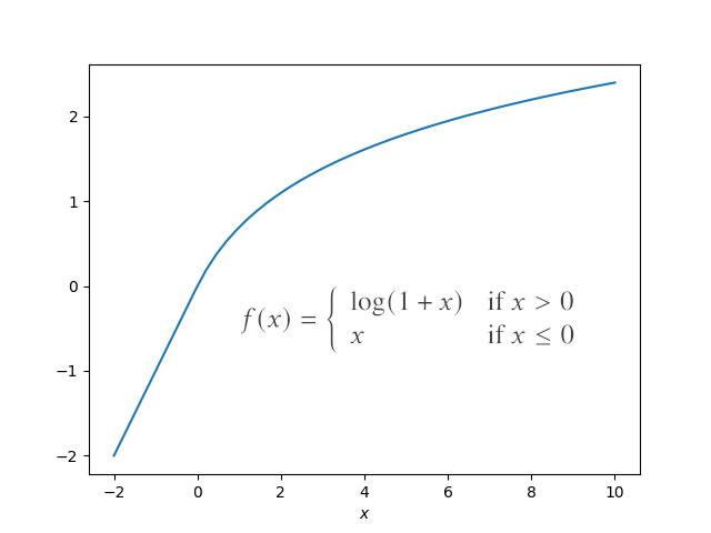
for negative x. The functions have a mediocre fit, which may be adequate for some applications, such as plotting data points, but not for others, such as visual design. Here’s a plot.

There’s something not quite smooth about the plot. It’s continuous, even differentiable, at 0, but still there’s sort of a kink at 0.

The way to quantify smoothness is to count how many times you can differentiate a function and have a continuous result. We would say the function above is C¹ but not C² because its first derivative is continuous but not differentiable. If two functions have the same number of derivatives, you can distinguish their smoothness by looking at the size of the derivatives. Or if you really want to get sophisticated, you can use Sobolev norms.

As a rule of thumb, your vision can detect a discontinuity in the second derivative, maybe the third derivative in some particularly sensitive contexts. For physical applications, you also want continuous second derivatives (acceleration). For example, you want a roller coaster track to be more than just continuous and once differentiable.

Natural cubic splines are often used in applications because they patch cubic polynomials together so that the result is C².

You can patch together smooth functions somewhat arbitrarily, but not analytic functions. If you wanted to extend the function log(1 + x) analytically, your only choice is log(1 + x). More on that here.

If you patch together a flat line and a circle, as in the corners of a rounded rectangle, the curve is continuous but not C². The second derivative jumps from 0 to 1/r where r is the radius of the circle. A squircle is similar to a rounded rectangle but has smoothly varying curvature.

Related posts

Log-ish

I saw a post online this morning that recomended the transformation

f(x) = \left\{ \begin{array}{ll} \log(1+x) & \mbox{if } x > 0 \\ x & \mbox{if } x \leq 0 \end{array} \right.

I could see how this could be very handy. Often you want something like a logarithmic scale, not for the exact properties of the logarithm but because it brings big numbers closer in. And for big values of x there’s little difference between log(x) and log(1 + x).

The function above is linear near the origin, literally linear for negative values and approximately linear for small positive values.

I’ve occasionally needed something like a log scale, but one that would handle values that dip below zero. This transformation would be good for that. If data were equally far above and below zero, I’d use something like arctangent instead.

Notice that the function has a noticeable bend around 0. The next post addresses this.

Uniformity increases entropy

Suppose you have a system with n possible states. The entropy of the system is maximized when all states are equally likely to occur. The entropy is minimized when one outcome is certain to occur.

You can say more. Starting from any set of probabilities, as you move in the direction of more uniformity, you increase entropy. And as you move in the direction of less uniformity, you decrease entropy.

These statements can be quantified and stated more precisely. That’s what the rest of this post will do.

***

Let pi be the probability of the ith state and let p be the vector of the pi.

\mathbf{p} = (p_1, p_2, \ldots, p_n)

Then the entropy of p is defined as

H(\mathbf{p}) = -\sum_{i=1}^n p_i \log_2 p_i

If one of the p‘s is 1 and the rest of the p‘s are zero, then H(p) = 0. (In the definition of entropy, 0 log2 0 is taken to be 0. You could justify this as the limit of x log2 x as x goes to zero.)

If each of the pi are equal, pi = 1/n, then H(p) = log2 n. The fact that this is the maximum entropy, and that compromises between the two extremes always decrease entropy, comes from the fact that the entropy function H is concave (proof). That is, if p1 is one list of probabilities and p2 another, then

H((1-\lambda) \mathbf{p}_1 + \lambda\mathbf{p}_2) \geq (1 - \lambda) H( \mathbf{p}_1) + \lambda H(\mathbf{p}_2)

When we speak informally of moving from p1 in the direction of p2, we mean we increase the parameter λ from 0 to some positive amount no more than 1.

Because entropy is concave, there are no local maxima. As you approach the location of global maximum entropy, i.e. equal state probabilities, from any direction, entropy increases monotonically.

Sinc function approximation

The sinc function

sinc(x) = sin(x) / x

comes up continually in signal processing. If x is moderately small, the approximation

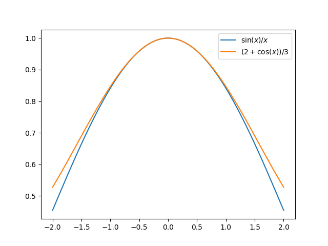
sinc(x) ≈ (2 + cos(x))/3

is remarkably good, with an error on the order of x4/180. This could be useful in situations where you’re working with the sinc function and the x in the denominator is awkward to deal with and you’d rather have a pure trig function.

Here’s a plot:

Of course the approximation is only good for small x. For large x the sinc function approaches zero while (2 + cos(x))/3 oscillates with constant amplitude forever.

When the approximation is good, it is very, very good, which reminds me of this nursery rhyme.

There was a little girl,
Who had a little curl,
Right in the middle of her forehead.
When she was good,
She was very, very good,
But when she was bad, she was horrid.

More sinc posts

Arithmetic for fun and profit

Four years ago I wrote a blog post about simple solutions to client problems. The post opens by recounting a conversation with a friend that ended with my friend saying “So, basically you’re recommending division.”

That conversation came back to me recently when I had a similar conversation during a deposition. I had to explain that the highly sophisticated method I used to arrive at a number in my report was to take the ratio of two other numbers.

I don’t always do division for clients. Sometimes I do multiplication, as when a lawyer asked me to compute the momentum of a car. There I had to multiply mass and velocity. (I actually turned down that project because I had a sense there was a lot more to the problem than I was being told.)

Of course real-world problems do not always have trivial solutions. Sometimes getting to the solution is complicated even though the solution itself is simple. And sometimes the solution is complicated because that’s just how things are. You might need something complicated, like a cepstrum analysis, or you might just need arithmetic.

Why use hash puzzles for proof-of-work?

A couple days ago I wrote about the the problem that Bitcoin requires to be solved as proof-of-work. In a nutshell, you need to tweak a block of transactions until the SHA256 double hash of its header is below a target value [1]. Not all cryptocurrencies use proof of work, but those that do mostly use hash-based puzzles.

Other cryptocurrencies use a different hashing problem, but they still use hashes. Litecoin and Dogecoin use the same proof-of-work problem, similar to the one Bitcoin uses, but with the scrypt (pronounced S-crypt) hash function. Several cryptocurrencies use a hashing problem based on Equihash. Monero uses its RandomX algorithm for proof-of-work, and although this algorithm has multiple components, it ultimately solves a hashing problem. [2]

Why hash puzzles?

Why do cryptocurrencies use hashing problems for proof of work? In principle they could use any computational problem that is hard to solve but easy to verify, such as numerous problems in computational number theory.

One reason is that computer scientists are confident that quantum computing would not reduce the difficulty of solving hash puzzles, even though it would reduce the difficulty of factoring-based puzzles. Also, there is general agreement that it’s unlikely a mathematical breakthrough will find a weakness in hashing functions.

Ian Cassels said “Cryptography is a mixture of mathematics and muddle, and without the muddle the mathematics can be used against you.” Hashing is much more muddle than mathematics.

Why not do something useful?

Hash puzzles work well for demonstrating work done, but they’re otherwise useless. They keep the wheels of cryptocurrencies turning, but the solutions themselves are intrinsically worthless.

Wouldn’t it be nice if crypto miners were solving useful problems like protein folding? You could do that. In fact there is a cryptocurrency FoldingCoin that does just that. But FoldingCoin has a market cap seven orders of magnitude smaller than Bitcoin, on the order of $200,000 compared to Bitcoin’s market cap of $2T.

Cryptocurrencies that use proof of useful work have not taken off. This might necessarily be the case. Requiring practical work creates divergent incentives. If you base a currency on the difficulty of protein folding computations, for example, it would cause major disruption if a pharmaceutical company decided to get into mining protein folding cryptocurrency at a loss because it values the results.

Going back to Cassels’ remark about mathematics and muddle, practical real-world problems often have a mathematical structure. Which is a huge blessing, except when you’re designing problems to be hard. Hash-based problems have gradually become easier to solve over time, and cryptocurrencies have adjusted. But a mathematical breakthrough for solving a practical problem would have the potential to disrupt a currency faster than the market could adapt.

Related posts

[1] You don’t change the transaction amounts, but you may change the order in which the transactions are arranged into a Merkle tree so that you get different hash values. You can also change a 32-bit nonce, and a timestamp, but most of the degrees of freedom you need in order to find an acceptable hash comes from rearranging the tree.

[2] Both scrypt and Equihash were designed to be memory intensive and to thwart the advantage custom ASIC mining hardware. However, people have found a way to use ASIC hardware to solve scrypt and Equihash problems. RandomX requires running a randomly generated problem before hashing the output in an attempt to frustrate efforts to develop specialized mining hardware.