Beta distribution with given mean and variance

It occurred to me recently that a problem I solved numerically years ago could be solved analytically, the problem of determining beta distribution parameters so that the distribution has a specified mean and variance. The calculation turns out to be fairly simple. Maybe someone has done it before.

Problem statement

The beta distribution has two positive parameters, a and b, and has probability density proportional to [1]

for x between 0 and 1.

The mean of a beta(a, b) distribution is

and the variance is

Given μ and σ² we want to solve for a and b. In order for the problem to be meaningful μ must be between 0 and 1, and σ² must be less than μ(1 − μ). [2]

As we will see shortly, these two necessary conditions for a solution are also sufficient.

Visualization

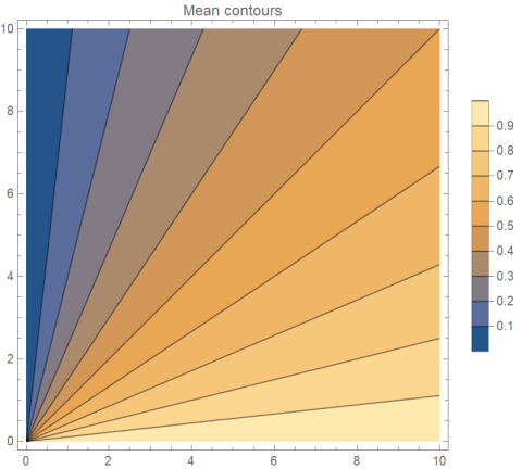
Graphically, we want to find the intersection of a line of constant mean

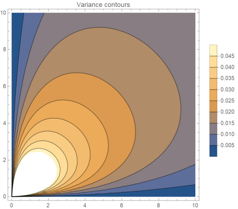
with a line of constant variance.

Note that the scales in the two plots differ.

Solution

If we set

then b = ka and so we can eliminate b from the equation for variance to get

Now since a > 0, we can divide by a²

and from there solve for a:

and b = ka.

We require σ² to be less than μ(1 − μ), or equivalently we require the ratio of μ(1 − μ) to σ² to be greater than 1. It works out that the solution a is the product of the mean and the amount by which the ratio of μ(1 − μ) to σ² exceeds 1.

Verification

Here is a little code to check for errors in the derivation above. It generates μ and σ² values at random, solves for a and b, then checks that the beta(a, b) distribution has the specified mean and variance.

    from scipy.stats import uniform, beta
    
    for _ in range(100):
        mu = uniform.rvs()
        sigma2 = uniform.rvs(0, mu*(1-mu))
    
        a = mu*(mu*(1-mu)/sigma2 - 1)
        b = a*(1-mu)/mu
    
        x = beta(a, b)
        assert( abs(x.mean() - mu) < 1e-10)
        assert( abs(x.var() - sigma2) < 1e-10)
    
    print("Done")

Related posts

• Determining a distribution from two quantiles
• Error in the normal approximation to a beta
• Diagram of probability distribution relationships

[1] It’s often easiest to think of probability densities ignoring proportionality constants. Densities integrate to 1, so the proportionality constants are determined by the rest of the expression for the density. In the case of the beta distribution, the proportionality constant works out to Γ(a + b) / Γ(a) Γ(b).

[2] The variance of a beta distribution factors into μ(1 − μ)/(a + b + 1), so it is less than μ(1 − μ).