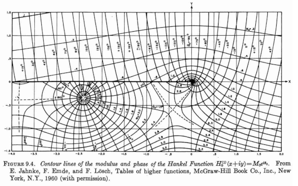
Abramowitz and Stegun has quite a few intriguing plots. The post will focus on the follow plot, Figure 9.4, available here.

We will explain what the plot is and approximately reproduce it.
The plot comes from the chapter on Bessel functions, but the caption says it is a plot of the Hankel function H0(1). Why a plot of a Hankel function and not a Bessel function? The Hankel functions are linear combinations of the Bessel functions of the first and second kind:
H0(1) = J0 + i Y0
More on that Hankel functions and their relations to Bessel functions here.
The plot is the overlay of two kinds of contour plots: one for lines of constant magnitude and one for lines of constant phase. That is, if the function values are written in the form reiθ then one plot shows lines of constant r and one plot shows lines of constant θ.
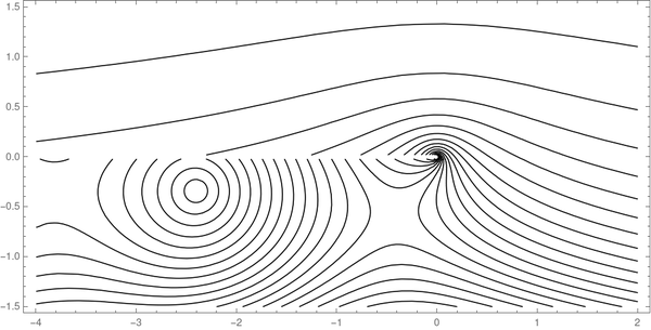
We can roughly reproduce the plot of magnitude contours with the following Mathematica command:
ContourPlot[Abs[HankelH1[0, x + I y]], {x, -4, 2 }, {y, -1.5 , 1.5 },
 Contours -> 20, ContourShading -> None, AspectRatio -> 1/2]
This produces the following plot.

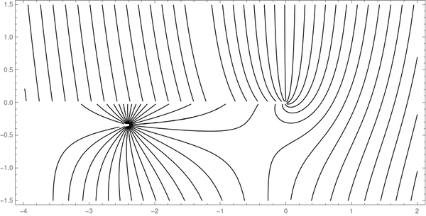
Similarly, we can replace Abs with Arg in the Mathematica command and increase Contours to 30 to obtain the following phase contour plot.

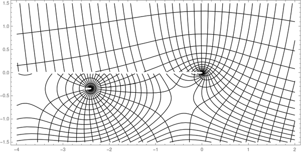
Finally, we can stack the two plots on top of each other using Mathematica’s Show command.

By the way, you can clearly see the branch cut in the middle. The Hankel function is continuous (even analytic) as you move clockwise from the second quadrant around to the third, but it is discontinuous across the negative real axis because of the branch cut.

You can also see missed contours where the argument is plus or minus 180