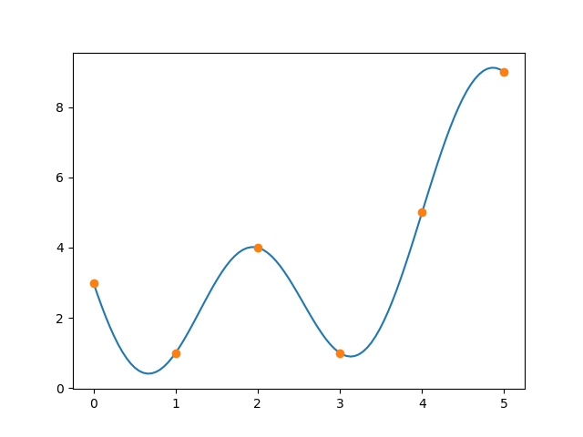
Suppose you want to interpolate a set of data points with a combination of sines and cosines.
One way to approach this problem would be to set up a system of equations for the coefficients of the sines and cosines. If you have N data points, you will get a system of N equations in N unknowns. The system will have a unique solution, though this is not obvious a priori.
Another approach would be to use the discrete Fourier transform (DFT). This is the approach that would commonly be used in practice. It’s even further from obvious a priori that this would work, but it does. (The DFT is so often computed using the FFT algorithm that the transform is often referred to by the algorithm name. If you’d like, mentally substitute FFT for DFT in the rest of the post.)
There are multiple ways to motivate the DFT, and the way suggested by the name is to derive the DFT as a discrete approximation to the (continuous) Fourier transform. Why should a discrete approximation to an integral transform also solve an interpolation problem? This doesn’t sound inevitable, or even plausible, but it is the case.
Another way to motivate the DFT is as the least-squares solution to fitting a sum of sines and cosines to a set of points. Since this is phrased as an optimization problem rather than an interpolation problem, it is clear that it will have a solution. However, it is not clear that the error in the optimal fit will in fact be zero. Furthermore, the equation for the coefficients in the solution is the same as the equation for the DFT. You can find a derivation in [1].
Example
Let’s take the vector [3, 1, 4, 1, 5, 9] and find trig functions that pass through these points. We can use the FFT as implemented in Python’s SciPy library to find a set of complex exponentials that pass through the points.
    from scipy.fft import fft
    from numpy import exp, array, pi, round

    x = array([3, 1, 4, 1, 5, 9])
    y = fft(x)

    N = len(x)
    z = [sum([exp(2j*pi*k*n/N)*y[k] for k in range(N)])/N for n in range(N)]
Aside from rounding errors on the order of 10−15 the vector z equals the vector x.
Turning the expression for z above into a mathematical expression, we have
f(z) = y0 + y1 exp(nπi/3) + y2 exp(2nπi/3) + y3 exp(nπi) + y4 exp(4nπi/3) + y5 exp(5nπi/3)
where the y‘s come from the FFT above.
To find sines and cosines we need to use Euler’s formula
exp(iθ) = cos(θ) + i sin(θ)
Because started with real data x, there will be symmetries in the FFT components x that simplify the reduction of the complex function f to a real-valued function g using sines and cosines; some of the components will be conjugate and so the complex parts cancel out.
6 g(x) = y0 + (y1 + y5) cos(πx/3) + (y2 + y4) cos(2πx/3) + y3 cos(πx)
+ i (y1 − y5) sin(πx/3) + (y2 − y4) cos(2πx/3)
and so
g(x) = 3.833 + 0.8333 cos(πx/3) − 1.833 cos(2πx/3) + 0.1666 cos(πx)
− 2.5981 sin(πx/3) − 2.0207 cos(2πx/3)
Here’s a plot that verifies that g(x) passes through the specified points.

Related posts
[1] William L. Briggs and Van Emden Henson. The DFT: An Owner’s Manual for the Discrete Fourier Transform. SIAM 1995.
