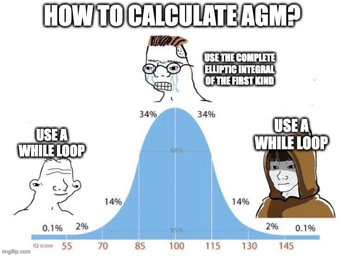
The last couple article have looked at various kinds of mean. The Python code for four of these means is trivial:
gm  = lambda a, b: (a*b)**0.5
am  = lambda a, b: (a + b)/2
hm  = lambda a, b: 2*a*b/(a+b)
chm = lambda a, b: (a**2 + b**2)/(a + b)
But the arithmetic-geometric mean (AGM) is not trivial:
from numpy import pi
from scipy.special import ellipk

agm = lambda a, b: 0.25*pi*(a + b)/ellipk((a - b)**2/(a + b)**2)
The arithmetic-geometric mean is defined by iterating the arithmetic and geometric means and taking the limit. This iteration converges very quickly, and so writing code that directly implements the definition is efficient.
But the AGM can also be computed via a special function K, the “complete elliptic integral of the first kind,” which makes the code above more compact. This is conceptually nice because we can think of the AGM as a simple function, not an iterative process.
But how is K evaluated? In some sense it doesn’t matter: it’s encapsulated in the SciPy library. But someone has to write SciPy. I haven’t looked at the SciPy source code, but usually K is calculated numerically using the AGM because, as we said above, the AGM converges very quickly.

This fits the pattern of a bell curve meme: the novice and expert approaches are the same, but for different reasons. The novice uses an iterative approach because that directly implements the definition. The expert knows about the elliptic integral, but also knows that the iterative approach suggested by the definition is remarkably efficient and eliminates the need to import a library.
Although it’s easy to implement the AGM with a while loop, the code above does have some advantages. For one thing, it pushes the responsibility for validation and exception handling onto the library. On the other hand, the code is easy to get wrong because there are two conventions on how to parameterize K and you have to be sure to use the same one your library uses.
