Visualizing real roots of a high degree polynomial

The previous post looked at finding the expected number of real zeros of high degree polynomials. If you wanted to see how many real roots a particular high degree polynomial has, you run into several difficulties.

If you use something like Descartes’ rule of signs, you’re likely to greatly over-estimate the number of roots. It would be easier to plot the function and look for the roots. But this brings up a couple more problems.

First, what range should you plot over? However far out you plot, how do you know there’s not another zero outside your plot?

Second, a high-degree polynomial is likely to vary by many orders of magnitude, making it impossible to see a plot on a single scale.

The first difficulty can be overcome by a theorem of Lagrange [1] that says all the zeros of an nth degree polynomial are contained in a disk of radius

centered at the origin of the complex plane. Here a_i is the coefficient of xⁱ.

The second difficulty can be overcome by plotting a transform of the polynomial rather than the polynomial itself. The hyperbolic tangent function works well because it maps 0 to 0, and because it compresses the real line into the interval (-1, 1). It will give a distorted picture of the polynomial, but it will preserve the zeros.

We will illustrate all this with some Python code.

We can evaluate our polynomial from an array of coefficients using Horner’s method.

    def poly(coeff, x):
        p = 0.0
        for c in reversed(coeff):
            p *= x
            p += c
        return p

Next, we generate the coefficients of a random 100th degree polynomial.

    import scipy as sp
    from scipy.stats import norm
 
    sp.random.seed(20201228) # today's date

    degree = 100
    coeff = norm.rvs(size = degree+1)

Now we find Lagrange’s bounds on the roots.

    m = max(1, sum(abs(coeff[:-2]/coeff[-1])))

Now we can plot the tanh of our polynomial

    import numpy as np
    import matplotlib.pyplot as plt

    x = np.linspace(-m, m, 1000)
    y = poly(coeff, x)
    z = np.tanh(y)
    plt.plot(x, z)

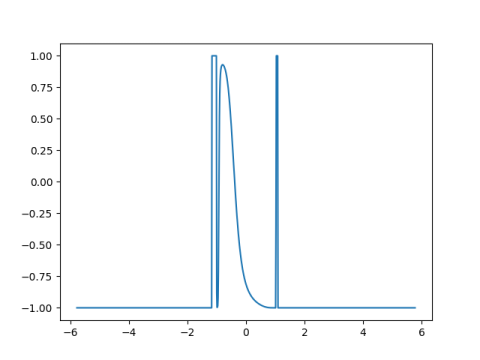
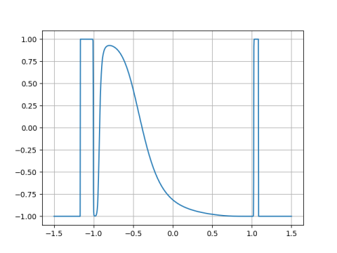
This produces a plot that’s basically just a spike. Lagrange’s bound is very generous in this case, but at least we know we’ve looked widely enough to start with. if we zoom in on the spike we get the following.

If we hadn’t taken the tanh our plot would vary by over 80 orders of magnitude.

We can zoom in a bit to see the zeros more clearly.

[1] Another bound on zeros due to Cauchy is

In this example, Cauchy’s bound is tighter. You could always compute both bounds and take the smaller bound.