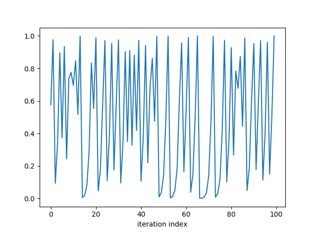
Iteration of the quadratic function f(x) = 4x(1-x) is a famous example in chaos theory. Here’s what the first few iterations look like, starting with 1/√3. (There’s nothing special about that starting point; any point that doesn’t iterate to exactly zero will do.)

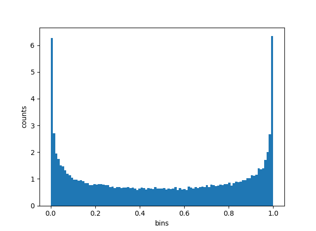
The values appear to bounce all over the place. Let’s look at a histogram of the sequence.

Indeed the points do bounce all over the unit interval, though they more often bounce near one of the ends.
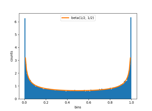
Does that distribution look familiar? You might recognize it from Bayesian statistics. It’s a beta distribution. It’s symmetric, so the two beta distribution parameters are equal. There’s a vertical asymptote on each end, so the parameters are less than 1. In fact, it’s a beta(1/2, 1/2) distribution. It comes up, for example, as the Jeffreys prior for Bernoulli trials.
The graph below adds the beta(1/2, 1/2) density to the histogram to show how well it fits.

We have to be careful in describing the relation between the iterations and the beta distribution. The iterates are ergodic, not random. The sequence of points does not simulate independent draws from any distribution: points near 0.5 are always sent to points near 1, points near 1 are always sent to points near 0, etc. But in aggregate, the points do fill out the unit interval like samples from a beta distribution. In the limit, the proportion of points in a region equals the probability of that region under a beta(1/2, 1/2) distribution.
Here’s the Python code that produced the graphs above.
import numpy as np
from scipy.stats import beta
import matplotlib.pyplot as plt

def quadratic(x):
    return 4*x*(1-x)

N = 100000
x = np.empty(N)

# arbitrary irrational starting point
x[0] = 1/np.sqrt(3)
for i in range(1, N):
    x[i] = quadratic( x[i-1] )

plt.plot(x[0:100])
plt.xlabel("iteration index")
plt.show()

t = np.linspace(0, 1, 100)
plt.hist(x, bins=t, normed=True)
plt.xlabel("bins")
plt.ylabel("counts")

plt.plot(t, beta(0.5,0.5).pdf(t), linewidth=3)
plt.legend(["beta(1/2, 1/2)"])
plt.show()

Very interesting! Thanks for this. I’d like to add that although the long-term spatial distribution of almost every orbit might appear to be Beta, the logistic map (with lambda=4) has periodic points of all periods (Sarkovskii’s Theorem). Therefore the density does depend on the initial condition and countably many points do not have that density. Even if your initial point is very close to a periodic point, the orbit will stay near the periodic orbit for many iterations, although ergodicity eventually wins. A good example is the initial condition 3/4+1e-12, which is close to the fixed point at x=3/4. The first 30-40 iterations stay close to the fixed point, and you can still see the effect in the histogram of the first 1000 iterations. So, as you say, don’t use this map as a random number generator!
let x = (1 – cos θ)/2; then 4 x ( 1 – x) = (1 – cos² θ) = 1 – (cos 2θ + 1) / 2 = (1-cos 2θ)/2 ; … for uniformly distributed θ ∈ [0,2π], the bits of (θ/2π) are iid Bernouli with mean 1/2; … QED.