Fair division and the Thue-Morse sequence

Suppose two captains, A and B, are choosing people for their teams. To make things fair, the two captains alternate choices: A, B, A, B, etc. This is much better than simply letting A choose his team first and leaving B the dregs, but it still gives A a substantial advantage. If each captain picks the best remaining player on each term, A will get the best player in each pair of choices.

How could we do better? One proposed strategy is the Thue-Morse sequence. Someone has to choose first, so let’s say it’s A. Then B chooses next. At this point A is still at an advantage, so we let B choose again before giving A the next pick. So the first four choices are ABBA. The next four choices reverse this: BAAB. Then the next eight choices reverse the pattern of the first eight choices. So the first 16 choices are ABBABAABBAABABBA. This process has been called “taking turns taking turns.”

In terms of 0’s and 1’s, the sequence is defined by t0 = 0, t2n = tn, and t2n+1 = 1 − t2n.

How well does this procedure work? Let’s simulate it by generating random values representing skill levels. We’ll sort the values and assign them to the two teams using the Thue-Morse sequence and look at the difference between the total point values on each team. Equivalently, we can sum the values, alternating the signs of the terms according to the Thue-Morse sequence.

    import numpy as np

    # Thue-Morse sequence
    TM  = np.array([1, -1, -1, 1])

    # Simple alternating signs
    Alt = np.array([1, -1, 1, -1])

    N = 1000000 # number of simulations

    y = TM # change y to Alt to swap out strategies
    total = 0
    for _ in range(N):
        x = sorted(np.random.random(4), reverse=True)
        total += sum(x*y)
    print(total/N)

When we use the alternating sequence, there’s an average skill difference between the two teams of around 0.4. This is a huge imbalance relative to expected total skill of 2. (Each skill is a uniform random value between 0 and 1, so the total skill of all four players is 2 on average.)

When we use the Thue-Morse sequence, the average difference in my simulation was 0.000144. With one million simulations, our results are good to about three decimal places [1], and so the difference is indistinguishable from 0 to the resolution of our simulation. (When I repeated the simulation I got -0.000635 as the average difference.)

There are several ways to explore this further. One would be to work out the exact expected values analytically. Another would be to look at distributions other than uniform.

* * *

[1] The error in the average of N simulations is on the order of 1/√N by the central limit theorem.

Positive polynomials and squares

If a real polynomial in one variable is a sum of squares, it obviously cannot be negative. For example, the polynomial

p(x) = (x2 − 3)2 + (x + 7)2

is obviously never negative for real values of x. What about the converse: If a real polynomial is never negative, is it a sum of squares? Yes, indeed it is.

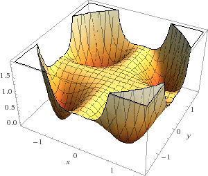
What about polynomials in two variables? There the answer is no. David Hilbert (1862–1943) knew that there must be positive polynomials that are not a sum of squares, but no one produced a specific example until Theodove Motzkin in 1967. His polynomial

p(x, y) = 1 − 3x2y2 + x2 y4 + x4 y2

is never negative but cannot be written as a sum of any number of squares. Here’s a plot:

Motzkin polynomial

Source: Single Digits


Sparsely populated zip codes

Country home

The dormitory I lived in as an undergraduate had its own five-digit zip code. It was rumored to be the largest dorm in the US, or maybe the largest west of the Mississippi, or something like that. There were about 3,000 of us living there. Although the dorm had enough people to justify its own zip code—some zip codes have far fewer people—zip code boundaries were later redraw so that the dorm shares its zip code with other areas.

Some zip code are so sparsely populated that people living in these areas are relatively easy to identify if you have other data. The so-called Safe Harbor provision of HIPAA (Health Insurance Portability and Accountability Act) says that it’s usually OK to include the first three digits of someone’s zip code in de-identified data. But there are some areas so thinly populated that even listing the first three digits of their zip code is considered too much of an identification risk.

Knowing that someone is part of an area containing 20,000 people hardly identifies them. The concern is that in combination with other information, zip code data is more informative in these areas.

2000 census

According to data from the 2000 census, the sparsely populated 3-digit zip code areas were

  • 036
  • 059
  • 063
  • 102
  • 203
  • 556
  • 692
  • 790
  • 821
  • 823
  • 830
  • 831
  • 878
  • 879
  • 884
  • 890
  • 893

2010 census

The list of sparsely populated zip codes is shorter now according to the 2010 census.

  • 036
  • 059
  • 102
  • 203
  • 205
  • 369
  • 556
  • 692
  • 821
  • 823
  • 878
  • 879
  • 884
  • 893

Zip codes 063, 790, 830, 831, and 890 dropped off the list, and zip codes 205 and 369 were added.

Speculation for 2020

It appears the list of sparsely populated zip codes has not changed since 2010 based on the 2017 American Community Survey. However, one should go by official census data rather than ACS data, and things could change between 2017 and 2020.

Related

Help with HIPAA de-identification

Category theory and Koine Greek

Fragment of the Gospel of John in Greek

When I was in college, I sat in on a communication workshop for Latin American preachers. This was unusual since I’m neither Latin American nor a preacher, but I’m glad I was there.

I learned several things in that workshop that I’ve used ever since. For example, when you’re gesturing about something moving forward in time, move your hand from left to right from the audience’s perspective. Since English speakers (and for the audience of this workshop, Spanish speakers) read from left to right, we think of time progressing from left to right. If you see someone talking about time moving forward, but you see motion from right to left, you feel a subtle cognitive dissonance. (Presumably you should reverse this when speaking to an audience whose primary language is Hebrew or Arabic.)

Another lesson from that workshop, the one I want to focus on here, is that you don’t always need to convey how you arrived at an idea. Specifically, the leader of the workshop said that if you discover something interesting from reading the New Testament in Greek, you can usually present your point persuasively using the text in your audience’s language without appealing to Greek. This isn’t always possible—you may need to explore the meaning of a Greek word or two—but you can use Greek for your personal study without necessarily sharing it publicly. The point isn’t to hide anything, only to consider your audience. In a room full of Greek scholars, bring out the Greek.

This story came up in a recent conversation with Brent Yorgey about category theory. You might discover something via category theory but then share it without discussing category theory. If your audience is well versed in category theory, then go ahead and bring out your categories. But otherwise your audience might be bored or intimidated, as many people would be listening to an argument based on the finer points of Koine Greek grammar. Microsoft’s LINQ software, for example, was inspired by category theory principles, but you’d be hard pressed to find any reference to this because most programmers don’t want to know or need to know where it came from. They just want to know how to use it.

Some things may sound profound when expressed in esoteric language, such as category theory or Koine Greek, that don’t seem so profound in more down-to-earth language. Expressing yourself in a different language helps filter out pedantry from useful ideas. (On the other hand, some things that looked like pure pedantry have turned out to be very useful. Some hairs are worth splitting.)

Sometimes you have to introduce a new terms because there isn’t a colloquial counterpart. Monads are a good example, a concept from category theory that has entered software development. A monad is what it is, and analogies to burritos and other foods don’t really help. Better to introduce the term and say plainly what it is.

More on applied category theory

New Twitter account for functional programming and categories

I’m starting a new Twitter account @FunctorFact for functional programming and category theory.

These two subjects have a lot of overlap, and some tweets will combine both, but many will be strictly about one or the other. So some content will be strictly about programming, some strictly about math, and some combining ideas from both.

FunctorFact icon

Prime factors, phone numbers, and the normal distribution

Telephone numbers typically have around three distinct prime factors.

The length of a phone number varies by country, but US a phone number is a 10 digit number, and 10-digit numbers are often divisible by three different prime numbers, give or take a couple. Assuming phone numbers are scattered among possible 10-digit numbers in a way that doesn’t bias their number of prime factors, these numbers will often have between 1 and 5 prime factors. If a country has 9- or 11-digit phone numbers, the result is essentially the same.

Let ω(n) be the number of distinct prime factors of n. Then the Erdős–Kac theorem says roughly that ω(n) is distributed like a normal random variable with mean and variance log log n. More precisely, fix two numbers a and b.  For a given value of x, count the proportion of positive integers less than x where

(ω(n) − log log n) / sqrt( log log n)

is between a and b. Then in the limit as x goes to infinity, this proportion approaches the probability that a standard normal random variable is between a and b.

So by that heuristic, the number of distinct prime factors of a 10-digit number is approximately normally distributed with mean and variance log log 10^11 = 3.232, and such a distribution is between 1 and 5 around 73% of the time.

My business phone number, for example, is 8324228646. Obviously this is divisible by 2. In fact it equals 2 × 32 × 462457147, and so it has exactly three distinct prime factors: 2, 3, and 462457147.

Here’s how you could play with this using Python.

    from sympy.ntheory import factorint

    def omega(n):
        return len(factorint(n))

I looked in SymPy and didn’t see an implementation of ω(n) directly, but it does have a function factorint that returns the prime factors of a number, along with their multiplicities, in a dictionary. So ω(n) is just the size of that dictionary.

I took the first 20 phone numbers in my contacts and ran them through omega and got results consistent with what you’d expect from the theory above. One was prime, and none had more than five factors.

Bar chart of umber of prime factors in a sample of phone numbers with heights [1, 3, 5, 8, 3]

Five lemma, ASCII art, and Unicode

A few days ago I wrote about creating ASCII art in Emacs using ditaa. Out of curiosity, I wanted to try making the Five Lemma diagram. [1]

The examples in the ditaa site all have arrows between boxes, but you don’t have to have boxes.

Here’s the ditaa source:

A₀ ---> A₁ ---> A₂ ---> A₃ ---> A₄
|       |       |       |       |            
| f₀    | f₁    | f₂    | f₃    | f₄    
|       |       |       |       |      
v       v       v       v       v      
B₀ ---> B₁ ---> B₂ ---> B₃ ---> B₄

and here’s the image it produces:

Five lemma diagram

It’s not pretty. You could make a nicer image with LaTeX. But as the old saying goes, the remarkable thing about a dancing bear is not that it dances well but that it dances at all.

The trick to getting the subscripts is to use Unicode characters 0x208n for subscript n. As I noted at the bottom of this post, ditaa isn’t strictly limited to ASCII art. You can use Unicode characters as well. You may or may not be able to see the subscripts in the source code they are not part of the most widely supported set of characters.

* * *

[1]  The Five Lemma is a diagram-chasing result from homological algebra. It lets you infer properties the middle function f from properties of the other f‘s.

Benford’s law, chi-square, and factorials

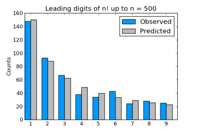
A while back I wrote about how the leading digits of factorials follow Benford’s law. That is, if you look at just the first digit of a sequence of factorials, they are not evenly distributed. Instead, 1’s are most popular, then 2’s, etc. Specifically, the proportion of factorials starting with n is roughly log10(1 + 1/n).

Someone has proved that the limiting distribution of leading digits of factorials exactly satisfies Benford’s law. But if we didn’t know this, we might use a chi-square statistic to measure how well the empirical results match expectations. As I argued in the previous post, statistical tests don’t apply here, but they can be useful anyway in giving us a way to measure the size of the deviations from theory.

Benford’s law makes a better illustration of the chi-square test than the example of prime remainders because the bins are unevenly sized, which they’re allowed to be in general. In the prime remainder post, they were all the same size.

The original post on leading digits of factorial explains why we compute the leading digits the way we do. Only one detail has changed: the original post used Python 2 and this one uses Python 3. Integer division was the default in Python 2, but now in Python 3 we have to use // to explicitly ask for integer division, floating point division being the new default.

Here’s a plot of the distribution of the leading digits for the first 500 factorials.

And here’s code to compute the chi-square statistic:

    from math import factorial, log10

    def leading_digit_int(n):
        while n > 9:
            n = n//10
        return n

    def chisq_stat(O, E):
        return sum( (o - e)**2/e for (o, e) in zip(O, E) )

    # Waste the 0th slot to make the code simpler.
    digits = [0]*10

    N = 500
    for i in range(N):
        digits[ leading_digit_int( factorial(i) ) ] += 1

    expected = [ N*log10(1 + 1/n) for n in range(1, 10) ]

    print( chisq_stat(digits[1:], expected) )

This gives a chi-square statistic of 7.693, very near the mean value of 8 for a chi-square distribution with eight degrees of freedom. (There are eight degrees of freedom, not nine, because if we know how many factorials start with the digits 1 through 8, we know how many start with 9.)

So the chi-square statistic suggests that the deviation from Benford’s law is just what we’d expect from random data following Benford’s law. And as we said before, this suggestion turns out to be correct.

Related posts

Hypothesis testing and number theory

This post uses a hypothesis test for proportions to look at a couple conjectures in number theory. It is similar to my earlier post on the chi-square test and prime remainders. You could read this as a post on statistics or a post on number theory, depending on which you’re less familiar with.

Using statistical tests on number theory problems is kind of odd. There’s nothing random going on, so in that sense the whole enterprise is unjustified. Nevertheless, statistical tests can be suggestive. They certainly don’t prove theorems, but they can give reason to suspect a theorem is true or false. In that sense, applying statistical tests to number theory isn’t all that different from applying them to more traditional settings.

First we’ll look at the remainders of primes modulo 4. Except for 2, all primes are odd, and so they either have remainder 1 or 3 when divided by 4. Brian Hayes wrote recently that Chebyshev noticed in the 1850’s that there seems to be more primes with remainder 3. Is the imbalance larger than one would expect to see from fair coin tosses?

Here’s some Python code to find the proportion of the first million primes (after 2) that have remainder 3 when divided by 4.

    from sympy import prime
    from scipy import sqrt

    n = 1000000
    rem3 = 0
    for i in range (2, n+2):
        if prime(i) % 4 == 3:
            rem3 += 1
    p_hat = rem3/n

This shows that of the first million odd primes, 500,202 are congruent to 3 mod 4. Would it be unusual for a coin to come up heads this many times in a million flips? To find out we’d compute the z-statistic:

z = \frac{\hat{p} - p}{\sqrt{pq/n}}

Here p is the proportion under the null hypothesis, q = 1 – p, and n is the sample size. In our case, the null hypothesis is p = 0.5 and n = 1,000,000. [1]

The code

    p = 0.5
    q = 1 - p
    z = (p_hat - p)/sqrt(p*q/n)

shows that z = 0.404, hardly a suspiciously large value. If we were looking at random values we’d see a z-score this large or larger 34% of the time. So in this case doesn’t suggest much.

***

[1] The derivation of the z statistic is fairly quick. If the proportion of successes is p, then the number of successes out of n trials is binomial(np). For large n, this is has approximately the same distribution as a normal distribution with the same mean and variance, mean np and variance npq. The proportion of successes then has approximately mean p and standard deviation √(pq/n). Subtracting the mean and dividing by the standard deviation normalizes the distribution to have mean 0 and variance 1. So under the null hypothesis, the z statistic has a standard normal distribution.