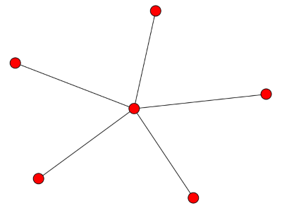
One way to get some understanding of a graph is to peel away nodes, starting with the least connected. The k-core of a graph is the maximal subgraph such that every vertex has degree at least k. The k-shell is the set of vertices that are part of the k-core but not part of the (k+1)-core.
For example, the 0-core of a graph is simply the entire graph since every vertex has at least zero edges; a vertex can’t have a negative number of edges. The 1-core of a graph contains the vertices that are connected to other vertices. You form the 1-core by throwing away the 0-shell, the set of isolated vertices. You move from the 1-core to the 2-core by removing nodes of degree 1 until everything that’s left has degree at least 2.
NB: You do not form the k-core simply by discarding nodes of degree less than k. For example, consider the star graph below.

If you peel off the nodes of degree 1, eventually you have nothing left. There is no 2-core, even though the original graph had a node of degree 5. Or going back to the definition, there is no subgraph such that every vertex has degree 2, and so no maximal subgraph. The node of degree 5 only has degree five because it is connected to nodes of degree 1.
The k-cores of a complete graph of degree n are simply the entire graph, for k ≤ n. The k-shells are empty for k < n.
Keyword overlap
Let’s see what the k-cores and k-shells look like for some more complex graphs. First, let’s go back to the post looking at the overlap in keywords. The edges of the graph are the 200 search terms that have lead visitors to the site at least twice. We connect two search terms if they share a word. The 56-core of the graph has 57 vertices, and the 57-core is empty. So the 56-core is a complete graph. Here’s the distribution of the k-shell sizes.

Random graphs
Next let’s look at a random graph. As in the post on spectra of random graphs, we look at an Erdős-Rényi graph Gn,p. First we start with n = 1000 and p = 0.01. So we start with 1000 nodes, and there’s a 0.01 that any particular pair of nodes is connected. Here are the core sizes for one such random graph:
[1000 1000 999 999 990 970 914 793]
So the 7-core has 793 nodes, then the 8-core is empty. I ran this ten times and the 7-core sizes ranged from size 709 to 849. But every time the 8-core was empty. The largest value of k such that the k-core is non-empty is called the degeneracy of the graph, so we could say the degeneracy was 7 every time.
I reran with n = 2000. The degeneracy was 14 every time. The 14-cores were in the range 1723 to 1810.
Finally I set n = 4000 and ran again. The degeneracy was 29 three times and 30 seven times. The final core sizes ranged from 3451 to 3714.
The experiments above suggest that the k-core size abruptly drops to zero, at a predictable value of k, and with a fairly predictable core size. There are papers on k-core size of random graphs, but I have not yet read any. (I have one in my to-read queue that someone let me know about after posting this article.)

That threshold value of k where the k-core becomes empty is called the degeneracy of the graph.
https://en.wikipedia.org/wiki/Degeneracy_(graph_theory)
There is a lot of work on using degeneracy to create fast algorithms.
Thanks, Austin. I updated the post to use “degeneracy” rather than my clunky wording.
Small note: If the 56-core of the graph has 57 vertices, it *is* the complete graph on 57 vertices (not *almost*, as you’ve written). The 56-core is, by definition, the maximal subgraph with minimum degree 56. For a vertex v to have degree 56 in that subgraph, there must be at least 57 vertices in it, v and its 56 neighbors. So v is adjacent to every other vertex in the 56-core. Since the 56-core has exactly 57 vertices, it is the complete graph K_{57}.
In general, the degeneracy of a graph on n nodes is at most n-1, and this bound is achieved uniquely by the complete graph.
Dane: You’re right. I had an off-by-one error in my head when I wrote “almost.”