Sometimes when people say they want random points, that’s not what they really want. Random points clump more than most people expect. Quasi-random sequences are not random in any mathematical sense, but they might match popular expectations of randomness better than the real thing, especially for aesthetic applications. If by “random” someone means “scattered around without a clear pattern and not clumped together” then quasi-random sequences might do the trick.
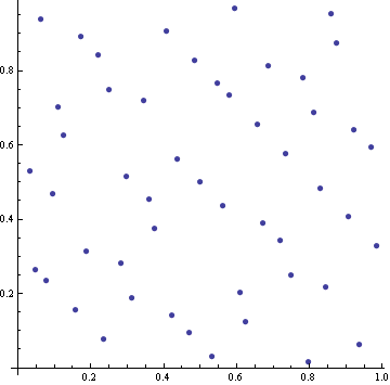
Here are the first 50 points in a quasi-random sequence of points in the unit square.

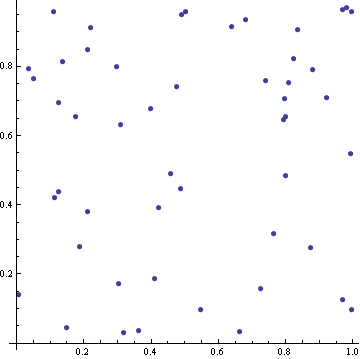
By contrast, here are 50 points in a unit square whose coordinates are uniform random samples.

The truly random points clump together. Notice the cluster of three points in the top right corner. There are few other instances of pairs of points being very close together. Also, there are fairly large areas that don’t contain any random points. The quasi-random points by contrast are better spread out. They have a self-avoiding property that keeps them from clustering, and they fill the space more efficiently.
Quasi-random sequences could be confused with pseudo-random sequences. They’re not at all the same thing. Pseudo-random sequences are computer-generated sequences that in many ways behave as if they were truly random, even though they were produced by deterministic algorithms. For many practical purposes, including sensitive statistical tests, pseudo-random sequences are simply random sequences. (The “truly” random points above were technically “pseudo-random” points.)
The quasi-random points above were part of a Sobol sequence, a common quasi-random sequence. Other quasi-random sequences include the Halton sequence and the Hammersley sequence. Mathematically, these sequences are defined has having low-discrepancy. Roughly speaking, this means the “discrepancy” between the number of points that actually fall in a volume and the number of points you’d expect to fall in the same volume is small. See the Wikipedia article on quasi-random sequences for more mathematical details.
Besides being aesthetically useful, quasi-random sequences are useful in applied mathematics. Because these sequences explore a space more efficiently than random sequences, quasi-random sequences sometimes lead to more efficient high-dimensional integration algorithms than Monte Carlo integration. Quasi-Monte Carlo integration, i.e. integration based on quasi-random sequences rather than random sequences, is popular in financial applications. Art Owen has written insightful papers on Quasi-Monte Carlo integration (QMC). He has classified which integration problems can be efficiently computed via QMC methods and which cannot. In a nutshell, QMC works well when the effective dimension of a problem is significantly lower than the actual dimension. For example, a financial model might ostensibly depend on 1000 variables, but 50 of those variables contribute far more to the integrand than all the other variables. The integrand might essentially be a function of only 50 variables. In that case, QMC will work well. Note that it is not necessary to identify these 50 variables or do any change of variables. QMC just magically takes advantage of the situation.
One disadvantage of QMC integration is that it doesn’t naturally lead to an estimate of its own accuracy, unlike Monte Carlo integration. Several hybrid approaches have been proposed to combine QMC integration and Monte Carlo integration to get the efficiency of the former and the error estimates of the latter. For example, one could randomly jitter the quasi-random points or randomly permute their components. Some of these results are in Art Owen’s papers.
To read more about quasi-random sequences, see the book Random Number Generation and Quasi-Monte Carlo Methods.

Thanks for this fascinating summary, John. Without really knowing it, I’ve been aiming for some quasi-random aesthetic effects. See the graphics here, for example, which I created by programatically nudging coordinates away from grid squares (using a random number generator). Maybe I should use a proper quasi-random sequence?
Here’s a fun post from a different blog (see the second footnote) which mentions trying to fill a screen with a flawed random number generator on the IBM PCJr:
http://www.wurb.com/stack/archives/530
Here’s a presentation from Ken Hanson describing other methods for generating sets of points. It starts off with digital halftoning algorithms and moves on from there.
Can we assess the quality / validity of the conclusions drawn from all laboratory experiments performed to date, which relied on a version of randomness, if we decide now that the randomness they used wasnt good enough? Exactly how does this new realization of quasi-randomness and the long established use of pseudo-randomness reflect / affect the quality of experimentation and the validity of its conclusions? Is it fair to look back on the history of science with doubtful contemplation?
Here is another question for you… a good one…
You say that there is a distinct difference between “true” randomness and what humans “feel” to be random. The latter being described as “quasi-random”.
Is it possible, then, to analyse a seemingly random set of data… and discern how random it is. To assess, based on “clumpage” and lack of “clumpage”, and decide whether or not the event truly was random… or if a human being tried to make it look random.
There are goodness of fit tests that will distinguish quasi-random sequences from random sequences.
Another realization I had. How do we know that quasi-random is merely appealing to human senses. How do we know that it isnt more true to randomness than what you deem “random”?
These pictures with the dots… they were generated on a computer, right? The regular “random” one wasnt truly random to begin with… it was pseudo-random, generated by a computer.
My observation is just that, which we deem random and which quasi-random is arbitrary, isnt it?
Could it be that the inherent “clumpiness” of “random” events is in fact the inherent pattern to be found in all pseudo-random generating algorithms? And that the unappealing nature of pseudo-random “randomness” is a legitimate concern?
Of course Im not suggesting that quasi-random is any less pseudo-random on a computer, but perhaps the algorithm has been adjusted, the outcomes modified, to be truer to actual random than you would like to believe. You presume that quasi-random only “looks” more random, and that clumpiness is actual random. But Im wondering if you have it right, if you just dont have too much faith in the computer.
Quasi-random sequences have aesthetic applications, but they can be objectively defined by their mathematical properties. For this reason they are sometimes called “low discrepancy sequences” where “discrepancy” has a technical definition.
I reached similar conclusions, not in art or integration, but on the theatrical stage. Turns out that when directors tell cast members to “go to a random position” on stage, they really mean “go to a quasi-random position.” For details, see
http://blogs.sas.com/content/iml/2011/01/28/random-uniform-versus-uniformly-spaced-applying-statistics-to-show-choir/