Valen Johnson and I recently posted a working paper on a method for stopping trials of ineffective drugs earlier. For Bayesians, we argue that our method is more consistently Bayesian than other methods in common use. For frequentists, we show that our method has better frequentist operating characteristics than the most commonly used safety monitoring method.
The paper looks at binary and time-to-event trials. The results are most dramatic for the time-to-event analog of the Thall-Simon method, the Thall-Wooten method, as shown below.

This graph plots the probability of concluding that an experimental treatment is inferior when simulating from true mean survival times ranging from 2 to 12 months. The trial is designed to test a null hypothesis of 6 months mean survival against an alternative hypothesis of 8 months mean survival. When the true mean survival time is less than the alternative hypothesis of 8 months, the Bayes factor design is more likely to stop early. And when the true mean survival time is greater than the alternative hypothesis, the Bayes factor method is less likely to stop early.
The Bayes factor method also outperforms the Thall-Simon method for monitoring single-arm trials with binary outcomes. The Bayes factor method stops more often when it should and less often when it should not. However, the difference in operating characteristics is not as pronounced as in the time-to-event case.
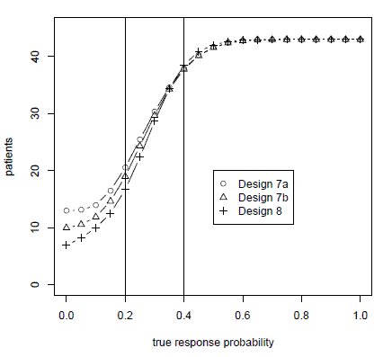
The paper also compares the Bayes factor method to the frequentist mainstay, the Simon two-stage design. Because the Bayes factor method uses continuous monitoring, the method is able to use fewer patients while maintaining the type I and type II error rates of the Simon design as illustrated in the graph below.

The graph above plots the number of patients used in a trial testing a null hypothesis of a 0.2 response rate against an alternative of a 0.4 response rate. Design 8 is the Bayes factor method advocated in the paper. Designs 7a and 7b are variations on the Simon two-stage design. The horizontal axis gives the true probabilities of response. We simulated true probabilities of response varying from 0 to 1 in increments of 0.05. The vertical axis gives the number of patients treated before the trial was stopped. When the true probability of response is less than the alternative hypothesis, the Bayes factor method treats fewer patients. When the true probability of response is better than the alternative hypothesis, the Bayes factor method treats slightly more patients.
Design 7a is the strict interpretation of the Simon method: one interim look at the data and another analysis at the end of the trial. Design 7b is the Simon method as implemented in practice, stopping when the criteria for continuing cannot be met at the next analysis. (For example, if the design says to stop if there are three or fewer responses out of the first 15 patients, then the method would stop after the 12th patient if there have been no responses.) In either case, the Bayes factor method uses fewer patients. The rejection probability curves, not shown here, show that the Bayes factor method matches (actually, slightly improves upon) the type I and type II error rates for the Simon two-stage design.
Related: Adaptive clinical trial design

It’s not a book on sequential analysis per se, but I’d recommend Jim Berger’s book on the likelihood principle.
Do you have any suggestions for books or review papers on application of Bayesian Statistics to sequential analysis? Thanks for any help on this matter.
In the first figure, it may be more informative to plot the difference between the curves. A plot such as you have gives some information about the relative difference that a plain difference plot would not have, but often plots like the one you present obscure differences, both in quality and quantity.
In this case the differences are easy to see, but often it is hard to see small differences between curves when they are simply overlaid, especially on slopes or shoulders of peaks.
Part of the reason for this is is the overall shape shared by both curves is a kind of noise when you consider the difference to be the signal.
But more significant I think is how we visually assess differences in curves. Our vision or mind tends to see the difference in parallell lines or curves to be the minimum distance between them, formed by a line segment perpendicular to both curves, rather than a difference in the Y axis direction.
So in the case of the figure above, the difference looks relatively small, maybe 0.1 or less, both in the region around 6 months and the region around 10 months. The difference in the region near 6 months looks like it balances out the difference near 10 months since they are in opposite direction. I think this is exascerbated by the proximity of the markers near 6 months — the circles seem to pair with the triangles which are one time unit in advance.
But the true difference looks to be much closer to 0.2 in the region near 6 months while the true difference near 10 months looks to be closer to 0.05. Those estimates are quite different. I suspect a plot of the differences would make that obvious.
Finally, I am glad you included 1.0 and especially 0.0 in the Y-axis, but I think a line at Y=0.0 would help. Towards 12 months it looks like the Bayes factor has a small but significantly non-zero probability of early stopping, with the Thall-Wooten having roughly twice the probability. But a closer look reveals that the Bayes factor probability is actually very close to 0 in that region.