The latest issue of Paged Out! has an article by Stephen Hewitt “An off-line backup of your cryptographic key using playing cards.” The idea is to use a deck of 52 to store a 128-bit cryptographic key. To erase the key, shuffle the deck. Hewitt gives his algorithm for embedding a key, one that can be carried out manually but isn’t maximally efficient.
You could store a 225-bit key as a permutation of 52 cards because
log2(52!) = 225.581.
But then how would you number permutations so you could go from a number to a particular permutation and later decode the permutation to a number? Is this even practical? For a small number n, you could encode a number k < n by enumerating the first k permutations of a set of n items, and you could decode by enumerating permutations until you find the one you have. But this is completely impractical for large n, such as n = 52.
The process of mapping permutation to an integer is called ranking, and the mapping from an integer to a permutation is called unranking. How efficiently can rankings and unrankings be calculated?
Let n be the number of symbols being permuted. Then there are simple algorithms for ranking and unranking with respect to lexicographical order that have complexity O(n²) and more sophisticated algorithms that have complexity O(n log n). There are also O(n) algorithms that do not preserve lexicographical order.
The Permutations class in SymPy has methods unrank_lex and rank to unrank and rank permutations according to lexicographical order.
The notation the Permutations class uses requires a little explanation. For example, suppose we unrank 2026.
>>> from sympy.combinatorics import Permutation
>>> Permutation.unrank_lex(52, 2026)
Permutation(45, 47, 51, 48, 46, 50)
The output is not a full list of 52 numbers in permuted order; it is only a cycle. The notation refers to the permutation that sends 45 to 47, 47 to 51, …, 50 to 45 and leaves everything else fixed.
If we rank the permutation given above, we get 2026 back.
>>> Permutation.rank(Permutation(45, 47, 51, 48, 46, 50))
2026
Note that we didn’t say how many elements (45, 47, 51, 48, 46, 50) is a permutation of. Because of lexicographical order, the rank would be the same whether we viewed this as a permutation of 52 objects or of more objects.
Now let’s do something larger. Let’s generate a 220-bit number and encode it as a permutation.
>>> n = random.getrandbits(225)
>>> a = Permutation.unrank_lex(52, n)
>>> n
40234719030664563684489051530416964877785781669439875437823431388841
>>> a
Permutation(0, 25, 32, 15, 8, 28)(1, 48, 34, 14, 10, 51, 38, 31, 21, 5, 42, 47, 29, 26, 46, 30, 50, 49, 37, 22, 18, 23)(2, 45, 17, 20, 36, 40, 11, 4, 7, 41, 33, 3, 43, 44, 19, 16, 35, 39, 12, 6, 9)
>>> Permutation.rank(a) == n
True
Now just for fun, let’s display the permutation above applied to a standard (French) deck of 52 cards. As explained here, symbols associated with these cards have a range of Unicode values. By printing these values, we can visualize the permuted deck.
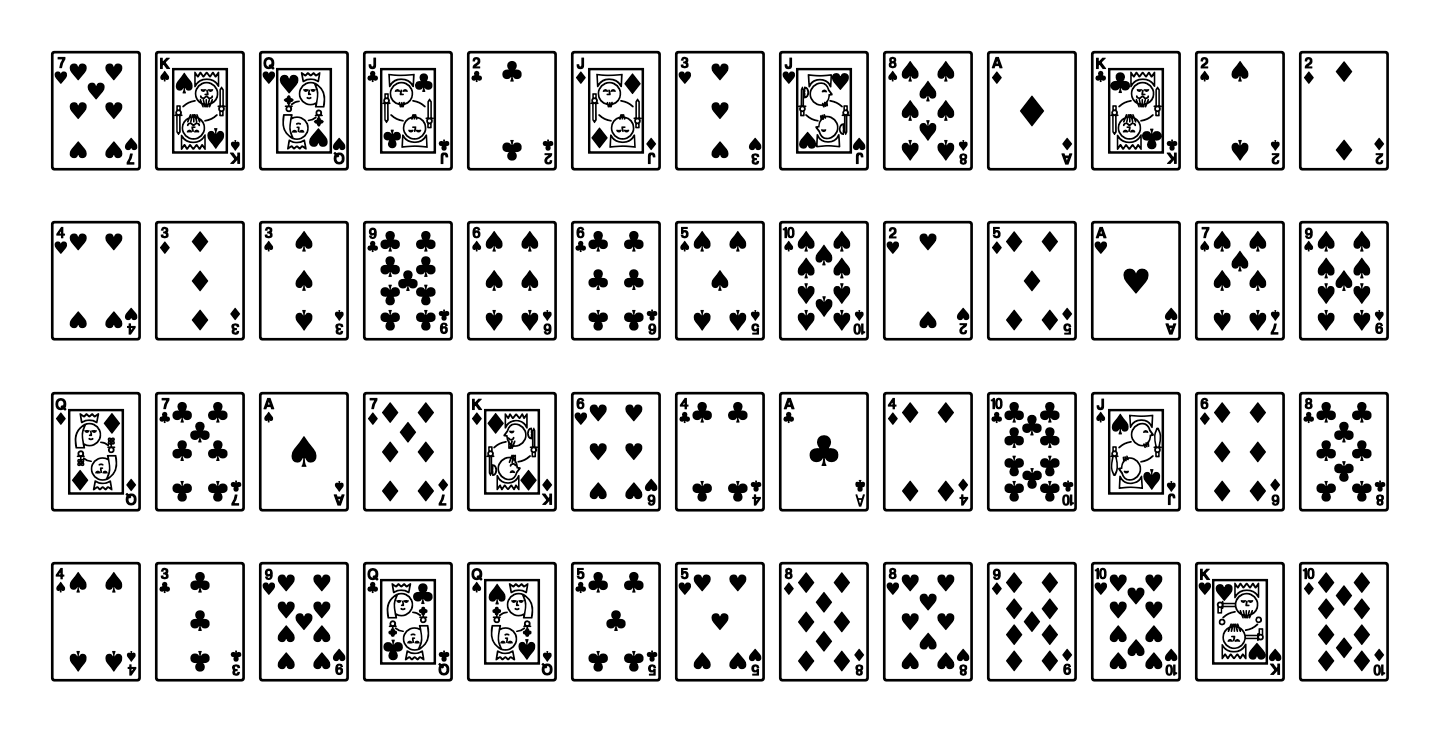
Here’s the code that made the image above.
spades = list(range(0x1F0A1, 0x1F0AF))
spades.remove(0x1F0AC) # take out the knight
cards = [s + 16*i for s in spades for i in range(4)]

a = Permutation.unrank_lex(52, n)
p = a(cards)

for i in range(4):
    for j in range(13):
        print(chr(p[13*i + j]), end="")
    print()
The code above is plenty fast, but Permutation has methods rank_nonlex and unrank_nonlex that run in O(n) time, which could be useful for n much larger than 52.

![\exp_q(x) = \sum_{n=0}^\infty [q \mid n] \frac{x^n}{n!} = \sum_{n=0}^\infty \frac{x^{nq}}{(nq)!}](https://www.johndcook.com/expq2.svg)

![\begin{align*} \frac{1}{q} \sum_{k=0}^{q-1} \exp(\omega^k x) &= \frac{1}{q} \sum_{k=0}^{q-1} \sum_{n=0}^\infty \frac{\omega^{kn}x^n}{n!} \\ &= \sum_{n=0}^\infty \left( \frac{1}{q} \sum_{k=0}^{q-1} \omega^{kn}\right) \frac{x^n}{n!} \\ &= \sum_{n=0}^\infty [q \mid n] \frac{x^n}{n!} \\ &= \exp_q(x) \end{align*}](https://www.johndcook.com/expq5.svg)
![\frac{1}{q} \sum_{k=0}^{q-1} \omega^{kn} = [q \mid n]](https://www.johndcook.com/expq6.svg)
